Window functions
Stingray now has a bunch of window functions that can be used for various applications in signal processing.
Windows available include: 1. Uniform or Rectangular Window 2. Parzen window 3. Hamming window 4. Hanning Window 5. Triangular window 6. Welch Window 7. Blackmann Window 8. Flat-top Window
All windows are available in stingray.utils package and called be used by calling create_window function. Below are some of the examples demonstrating different window functions.
[64]:
from stingray.utils import create_window

from scipy.fftpack import fft, fftshift, fftfreq
import numpy as np

import matplotlib.pyplot as plt
%matplotlib inline
create_window function in stingray.utils takes two parameters.
N: Number of data points in the windowwindow_type: Type of window to create. Default isuniform.
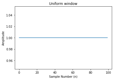
Uniform Window
[65]:
N = 100
window = create_window(N)
[66]:
plt.plot(window)
plt.title("Uniform window")
plt.ylabel("Amplitude")
plt.xlabel("Sample Number (n)")
[66]:
<matplotlib.text.Text at 0x21d8f0ccc50>
[67]:
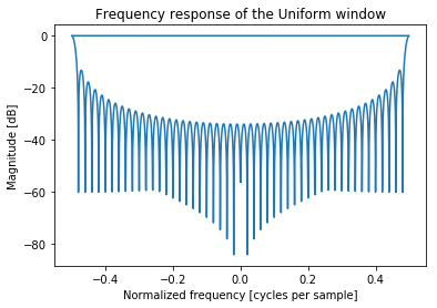
nfft = 2048
A = fft(window,nfft ) / (len(window)/2.0)
freq = fftfreq(nfft)
response = 20 * np.log10(np.abs(fftshift(A/(abs(A).max()))))
plt.plot(freq, response)
plt.title("Frequency response of the Uniform window")
plt.ylabel("Magnitude [dB]")
plt.xlabel("Normalized frequency [cycles per sample]")
C:\Users\Haroon Rashid\Anaconda3\lib\site-packages\ipykernel\__main__.py:4: RuntimeWarning: divide by zero encountered in log10
[67]:
<matplotlib.text.Text at 0x21d8f1b6e10>
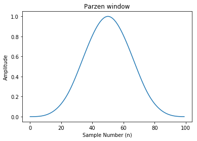
Parzen Window
[68]:
N = 100
window = create_window(N, window_type='parzen')
[69]:
plt.plot(window)
plt.title("Parzen window")
plt.ylabel("Amplitude")
plt.xlabel("Sample Number (n)")
[69]:
<matplotlib.text.Text at 0x21d8f1a8160>
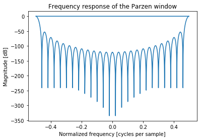
[70]:
nfft = 2048
A = fft(window,nfft ) / (len(window)/2.0)
freq = fftfreq(nfft)
response = 20 * np.log10(np.abs(fftshift(A/(abs(A).max()))))
plt.plot(freq, response)
plt.title("Frequency response of the Parzen window")
plt.ylabel("Magnitude [dB]")
plt.xlabel("Normalized frequency [cycles per sample]")
[70]:
<matplotlib.text.Text at 0x21d8f24b978>
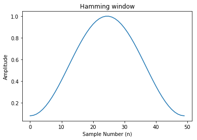
Hamming Window
[71]:
N = 50
window = create_window(N, window_type='hamming')
[72]:
plt.plot(window)
plt.title("Hamming window")
plt.ylabel("Amplitude")
plt.xlabel("Sample Number (n)")
[72]:
<matplotlib.text.Text at 0x21d8f360ba8>
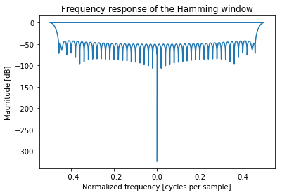
[73]:
nfft = 2048
A = fft(window,nfft ) / (len(window)/2.0)
freq = fftfreq(nfft)
response = 20 * np.log10(np.abs(fftshift(A/(abs(A).max()))))
plt.plot(freq, response)
plt.title("Frequency response of the Hamming window")
plt.ylabel("Magnitude [dB]")
plt.xlabel("Normalized frequency [cycles per sample]")
[73]:
<matplotlib.text.Text at 0x21d8f2f6fd0>
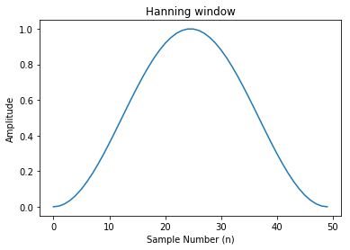
Hanning Window
[74]:
N = 50
window = create_window(N, window_type='hanning')
[75]:
plt.plot(window)
plt.title("Hanning window")
plt.ylabel("Amplitude")
plt.xlabel("Sample Number (n)")
[75]:
<matplotlib.text.Text at 0x21d8f34f470>
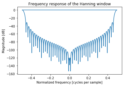
[76]:
nfft = 2048
A = fft(window,nfft ) / (len(window)/2.0)
freq = fftfreq(nfft)
response = 20 * np.log10(np.abs(fftshift(A/(abs(A).max()))))
plt.plot(freq, response)
plt.title("Frequency response of the Hanning window")
plt.ylabel("Magnitude [dB]")
plt.xlabel("Normalized frequency [cycles per sample]")
C:\Users\Haroon Rashid\Anaconda3\lib\site-packages\ipykernel\__main__.py:4: RuntimeWarning: divide by zero encountered in log10
[76]:
<matplotlib.text.Text at 0x21d8f4715f8>
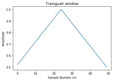
Traingular Window
[77]:
N = 50
window = create_window(N, window_type='triangular')
[78]:
plt.plot(window)
plt.title("Traingualr window")
plt.ylabel("Amplitude")
plt.xlabel("Sample Number (n)")
[78]:
<matplotlib.text.Text at 0x21d8f4397b8>
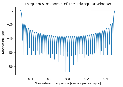
[79]:
nfft = 2048
A = fft(window,nfft ) / (len(window)/2.0)
freq = fftfreq(nfft)
response = 20 * np.log10(np.abs(fftshift(A/(abs(A).max()))))
plt.plot(freq, response)
plt.title("Frequency response of the Triangular window")
plt.ylabel("Magnitude [dB]")
plt.xlabel("Normalized frequency [cycles per sample]")
[79]:
<matplotlib.text.Text at 0x21d8f534470>
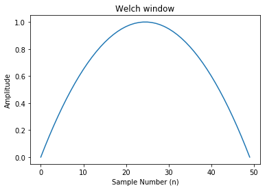
Welch Window
[80]:
N = 50
window = create_window(N, window_type='welch')
[81]:
plt.plot(window)
plt.title("Welch window")
plt.ylabel("Amplitude")
plt.xlabel("Sample Number (n)")
[81]:
<matplotlib.text.Text at 0x21d8f629eb8>
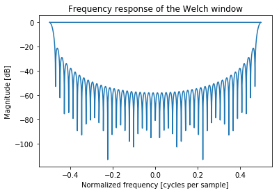
[82]:
nfft = 2048
A = fft(window,nfft ) / (len(window)/2.0)
freq = fftfreq(nfft)
response = 20 * np.log10(np.abs(fftshift(A/(abs(A).max()))))
plt.plot(freq, response)
plt.title("Frequency response of the Welch window")
plt.ylabel("Magnitude [dB]")
plt.xlabel("Normalized frequency [cycles per sample]")
C:\Users\Haroon Rashid\Anaconda3\lib\site-packages\ipykernel\__main__.py:4: RuntimeWarning: divide by zero encountered in log10
[82]:
<matplotlib.text.Text at 0x21d8f738080>
Blackmann’s Window
[83]:
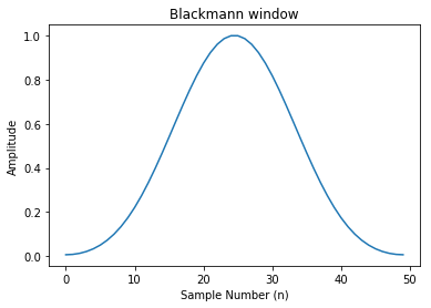
N = 50
window = create_window(N, window_type='blackmann')
[84]:
plt.plot(window)
plt.title("Blackmann window")
plt.ylabel("Amplitude")
plt.xlabel("Sample Number (n)")
[84]:
<matplotlib.text.Text at 0x21d8f6b92e8>
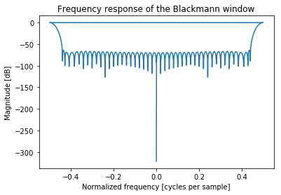
[85]:
nfft = 2048
A = fft(window,nfft ) / (len(window)/2.0)
freq = fftfreq(nfft)
response = 20 * np.log10(np.abs(fftshift(A/(abs(A).max()))))
plt.plot(freq, response)
plt.title("Frequency response of the Blackmann window")
plt.ylabel("Magnitude [dB]")
plt.xlabel("Normalized frequency [cycles per sample]")
[85]:
<matplotlib.text.Text at 0x21d9083b2e8>
Flat Top Window
[86]:
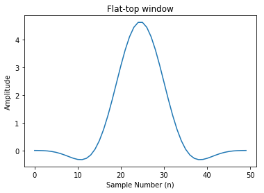
N = 50
window = create_window(N, window_type='flat-top')
[87]:
plt.plot(window)
plt.title("Flat-top window")
plt.ylabel("Amplitude")
plt.xlabel("Sample Number (n)")
[87]:
<matplotlib.text.Text at 0x21d9081e470>
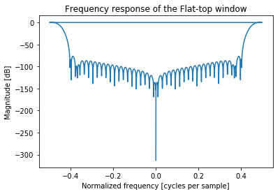
[88]:
nfft = 2048
A = fft(window,nfft ) / (len(window)/2.0)
freq = fftfreq(nfft)
response = 20 * np.log10(np.abs(fftshift(A/(abs(A).max()))))
plt.plot(freq, response)
plt.title("Frequency response of the Flat-top window")
plt.ylabel("Magnitude [dB]")
plt.xlabel("Normalized frequency [cycles per sample]")
[88]:
<matplotlib.text.Text at 0x21d909314a8>