Contents
This notebook covers the basics of creating TransferFunction object, obtaining time and energy resolved responses, plotting them and using IO methods available. Finally, artificial responses are introduced which provide a way for quick testing.
Setup
Set up some useful libraries.
[1]:
import numpy as np
from matplotlib import pyplot as plt
%matplotlib inline
Import relevant stingray libraries.
[2]:
from stingray.simulator.transfer import TransferFunction
from stingray.simulator.transfer import simple_ir, relativistic_ir
Creating TransferFunction
A transfer function can be initialized by passing a 2-d array containing time across the first dimension and energy across the second. For example, if the 2-d array is defined by arr, then arr[1][5] defines a time of 5 units and energy of 1 unit.
For the purpose of this tutorial, we have stored a 2-d array in a text file named intensity.txt. The script to generate this file is explained in Data Preparation notebook.
[3]:
response = np.loadtxt('intensity.txt')
Initialize transfer function by passing the array defined above.
[4]:
transfer = TransferFunction(response)
transfer.data.shape
[4]:
(524, 744)
By default, time and energy spacing across both axes are set to 1. However, they can be changed by supplying additional parameters dt and de.
Obtaining Time-Resolved Response
The 2-d transfer function can be converted into a time-resolved/energy-averaged response.
[5]:
transfer.time_response()
This sets time parameter which can be accessed by transfer.time
[6]:
transfer.time[1:10]
[6]:
array([0., 0., 0., 0., 0., 0., 0., 0., 0.])
Additionally, energy interval over which to average, can be specified by specifying e0 and e1 parameters.
Obtaining Energy-Resolved Response
Energy-resolved/time-averaged response can be also be formed from 2-d transfer function.
[7]:
transfer.energy_response()
This sets energy parameter which can be accessed by transfer.energy
[8]:
transfer.energy[1:10]
[8]:
array([0., 0., 0., 0., 0., 0., 0., 0., 0.])
Plotting Responses
TransferFunction() creates plots of time-resolved, energy-resolved and 2-d responses. These plots can be saved by setting save parameter.
[9]:
transfer.plot(response='2d')
[10]:
transfer.plot(response='time')
[11]:
transfer.plot(response='energy')
By enabling save=True parameter, the plots can be also saved.
IO
TransferFunction can be saved in pickle format and retrieved later.
[12]:
transfer.write('transfer.pickle')
Saved files can be read using static read() method.
[13]:
transfer_new = TransferFunction.read('transfer.pickle')
transfer_new.time[1:10]
[13]:
array([0., 0., 0., 0., 0., 0., 0., 0., 0.])
Artificial Responses
For quick testing, two helper impulse response models are provided.
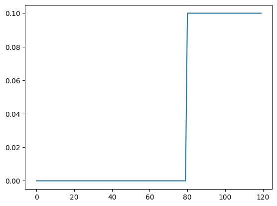
1- Simple IR
simple_ir() allows to define an impulse response of constant height. It takes in time resolution starting time, width and intensity as arguments.
[14]:
s_ir = simple_ir(dt=0.125, start=10, width=5, intensity=0.1)
plt.plot(s_ir)
[14]:
[<matplotlib.lines.Line2D at 0x2a22c0a90>]
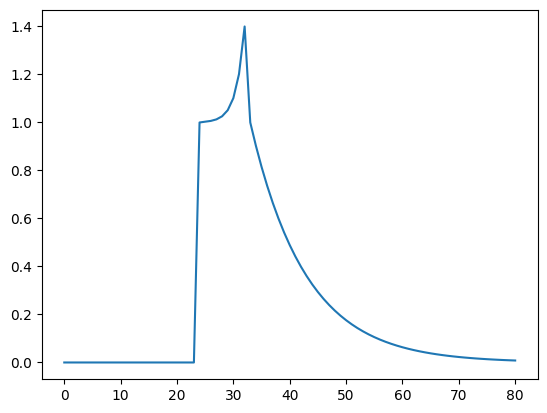
2- Relativistic IR
A more realistic impulse response mimicking black hole dynamics can be created using relativistic_ir(). Its arguments are: time_resolution, primary peak time, secondary peak time, end time, primary peak value, secondary peak value, rise slope and decay slope. These paramaters are set to appropriate values by default.
[15]:
r_ir = relativistic_ir(dt=0.125)
plt.plot(r_ir)
[15]:
[<matplotlib.lines.Line2D at 0x2a288ec20>]