Stingray Simulator (stingray.simulator)
Introduction
stingray.simulator provides a framework to simulate light curves with given variability distributions. In time series experiments, understanding the certainty is crucial to interpret the derived results in context of physical models. The simulator module provides tools to assess this uncertainty by simulating time series and spectral data.
Stingray simulator supports multiple methods to carry out these simulation. Light curves can be simulated through power-law spectrum, through a user-defined or pre-defined model, or through impulse responses. The module is designed in a way such that all these methods can be accessed using similar set of commands.
Note
stingray.simulator is currently a work-in-progress, and thus it is likely
there will still be API changes in later versions of Stingray. Backwards
compatibility support between versions will still be maintained as much as
possible, but new features and enhancements are coming in future versions.
Getting started
The examples here assume that the following libraries and modules have been imported:
>>> import numpy as np
>>> from stingray import Lightcurve, sampledata
>>> from stingray.simulator import simulator, models
Creating a Simulator Object
Stingray has a simulator class which can be used to instantiate a simulator object and subsequently, perform simulations. We can pass on arguments to this class class to set the properties of the desired light curve.
The simulator object can be instantiated as:
>>> sim = simulator.Simulator(N=1024, mean=0.5, dt=0.125, rms=1.0)
Here, N specifies the bins count of the simulated light curve, mean specifies
the mean value, dt is the time resolution, and rms is the fractional rms amplitude,
defined as the ratio of standard deviation to the mean.. Additional arguments can be
provided e.g. to account for the effect of red noise leakage.
Simulate Method
Stingray provides multiple ways to simulate a light curve. However, all these methods follow a common recipe:
>>> sim = simulator.Simulator(N=1024, mean=0.5, dt=0.125, rms=1.0)
>>> lc = sim.simulate(2)
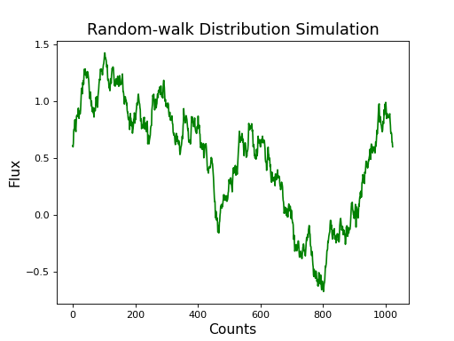
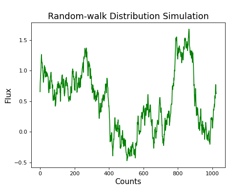
Using Power-Law Spectrum
When only an integer argument (beta) is provided to the simulate method, that integer defines the shape of the power law spectrum. Passing beta as 1 gives a flicker-noise distribution, while a beta of 2 generates a random-walk distribution.
from matplotlib import rcParams
rcParams['font.family'] = 'sans-serif'
rcParams['font.sans-serif'] = ['Tahoma']

import matplotlib.pyplot as plt
from stingray.simulator import simulator

# Instantiate simulator object
sim = simulator.Simulator(N=1024, mean=0.5, dt=0.125, rms=1.0)
# Specify beta value
lc = sim.simulate(2)

plt.plot(lc.counts, 'g')
plt.title('Random-walk Distribution Simulation', fontsize='16')
plt.xlabel('Counts', fontsize='14', )
plt.ylabel('Flux', fontsize='14')
plt.show()
(Source code, png, hires.png, pdf)
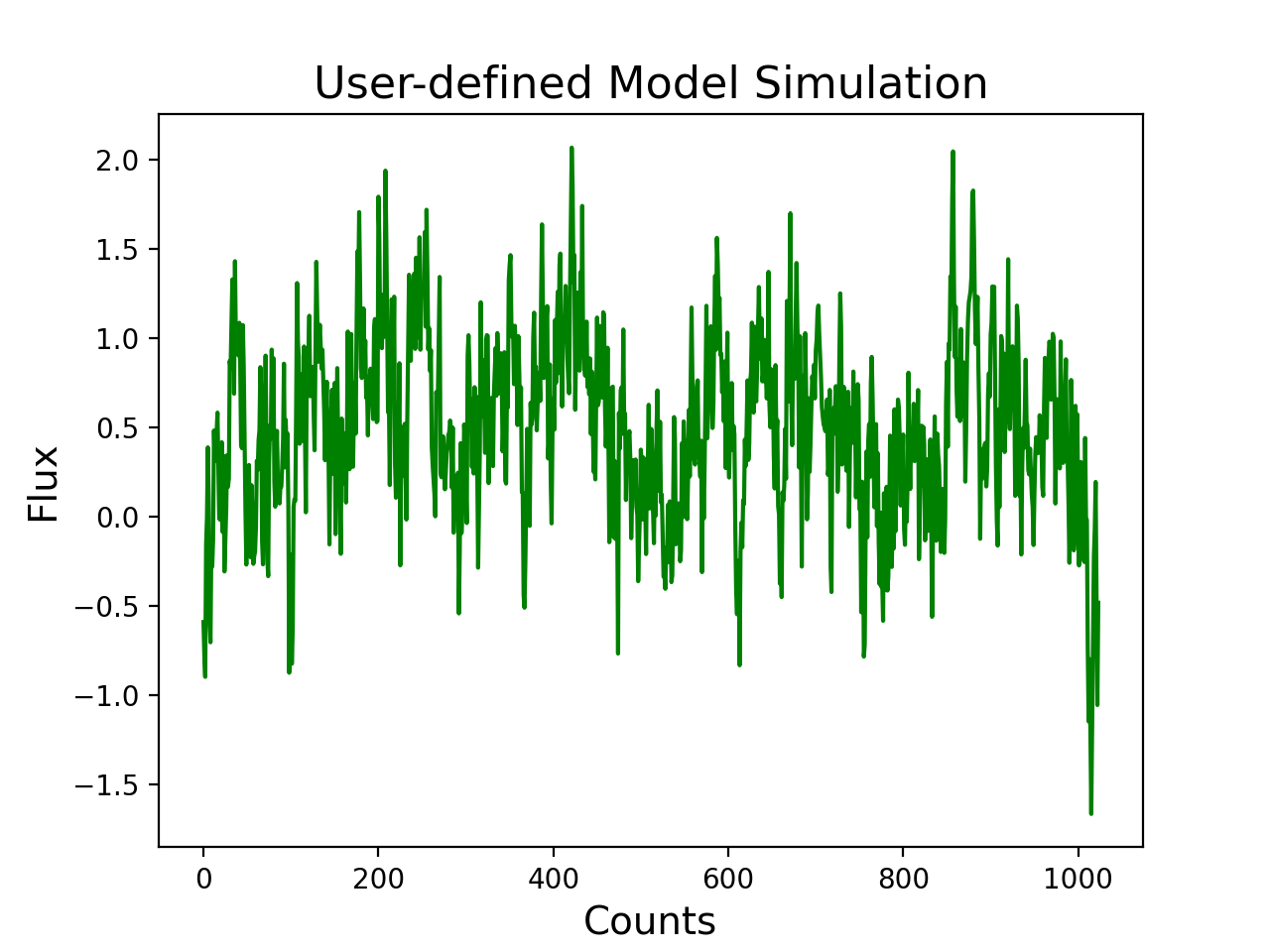
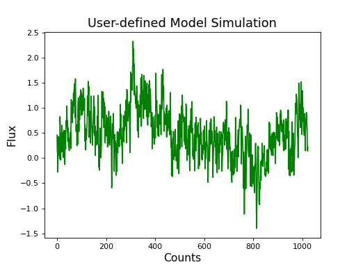
Using User-defined Model
Light curve can also be simulated using a user-defined spectrum, which can be passed on as a numpy array.
from matplotlib import rcParams
rcParams['font.family'] = 'sans-serif'
rcParams['font.sans-serif'] = ['Tahoma']

import matplotlib.pyplot as plt
from stingray.simulator import simulator

# Instantiate simulator object
sim = simulator.Simulator(N=1024, mean=0.5, dt=0.125, rms=1.0)
# Define a spectrum
w = np.fft.rfftfreq(sim.N, d=sim.dt)[1:]
spectrum = np.power((1/w),2/2)
# Simulate
lc = sim.simulate(spectrum)

plt.plot(lc.counts, 'g')
plt.title('User-defined Model Simulation', fontsize='16')
plt.xlabel('Counts', fontsize='14')
plt.ylabel('Flux', fontsize='14')
plt.show()
(Source code, png, hires.png, pdf)
Using Pre-defined Models
One of the pre-defined spectrum models can be used to simulate a light curve. In this case, model name and model parameters (as list iterable) need to be passed on as function arguments.
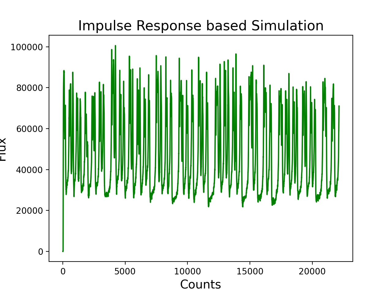
Using Impulse Response
In order to simulate a light curve using impulse response, we need the original light curve and impulse response. Stingray provides TransferFunction class which can be used to obtain time and energy averaged impulse response by passing in a 2-D intensity profile as the input. A detailed tutorial on obtaining impulse response is provided here.
Here, for the sake of simplicity, we use a simulated impulse response.
from matplotlib import rcParams
rcParams['font.family'] = 'sans-serif'
rcParams['font.sans-serif'] = ['Tahoma']

import matplotlib.pyplot as plt
from stingray import sampledata
from stingray.simulator import simulator

# Obtain a sample light curve
lc = sampledata.sample_data().counts
# Instantiate simulator object
sim = simulator.Simulator(N=1024, mean=0.5, dt=0.125, rms=1.0)
# Obtain an artificial impulse response
ir = sim.relativistic_ir()
# Simulate
lc_new = sim.simulate(lc, ir)

plt.plot(lc_new.counts, 'g')
plt.title('Impulse Response based Simulation', fontsize='16')
plt.xlabel('Counts', fontsize='14')
plt.ylabel('Flux', fontsize='14')
plt.show()
(Source code, png, hires.png, pdf)
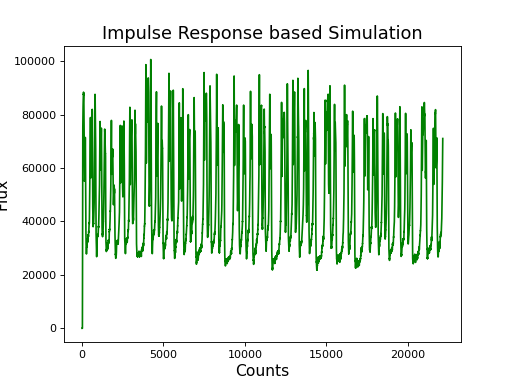
Since, the new light curve is produced by the convolution of original light curveand impulse response, its length is truncated by default for ease of analysis. This can be changed, however, by supplying an additional parameter full. However, at times, we do not need to include lag delay portion in the output light curve. This can be done by changing the final function parameter to filtered. For a more detailed analysis on lag-frequency spectrum, follow the notebook here.
Channel Simulation
The simulator class provides the functionality to simulate light curves independently for each channel. This is useful, for example, when dealing with energy dependent impulse responses where we can create a di↵erent simulation channel for each energy range. The module provides options to count, retrieve and delete channels.:
>>> sim = simulator.Simulator(N=1024, mean=0.5, dt=0.125, rms=1.0)
>>> sim.simulate_channel('3.5 - 4.5', 2)
>>> sim.count_channels()
1
>>> lc = sim.get_channel('3.5 - 4.5')
>>> sim.delete_channel('3.5 - 4.5')
Alternatively, assume that we have light curves in the simulated energy channels 3.5 - 4.5, 4.5 - 5.5 and 5.5 - 6.5. These channels can be retrieved or deleted in single commands.
>>> sim.count_channels()
0
>>> sim.simulate_channel('3.5 - 4.5', 2)
>>> sim.simulate_channel('4.5 - 5.5', 2)
>>> sim.simulate_channel('5.5 - 6.5', 2)
>>> chans = sim.get_channels(['3.5 - 4.5','4.5 - 5.5','5.5 - 6.5'])
>>> sim.delete_channels(['3.5 - 4.5','4.5 - 5.5','5.5 - 6.5'])