Contents
This notebook covers the basics of initializing and using the functionalities of simulator class. Various ways of simulating light curves that include ‘power law distribution’, ‘user-defined responses’, ‘pre’defined responses’ and ‘impulse responses’ are covered. The notebook also illustrates channel creation and ways to store and retrieve simulator objects.
Setup
Import some useful libraries.
[1]:
%load_ext autoreload
%autoreload 2
import numpy as np
from matplotlib import pyplot as plt
%matplotlib inline
Import relevant stingray libraries.
[2]:
from stingray import Lightcurve, Crossspectrum, sampledata, Powerspectrum
from stingray.simulator import simulator, models
from stingray.fourier import poisson_level
Creating a Simulator Object
Stingray has a simulator class which can be used to instantiate a simulator object and subsequently, perform simulations. Arguments can be passed in Simulator class to set the properties of simulated light curve.
In this case, we instantiate a simulator object specifying the number of data points in the output light curve, the expected mean and binning interval.
[3]:
sim = simulator.Simulator(N=10000, mean=5, rms=0.4, dt=0.125, red_noise=8, poisson=False)
sim_pois = simulator.Simulator(N=10000, mean=5, rms=0.4, dt=0.125, red_noise=8, poisson=True)
We also import some sample data for later use.
[4]:
sample = sampledata.sample_data().counts
Light Curve Simulation
There are multiple way to simulate a light curve:
Using
power-lawspectrumUsing user-defined model
Using pre-defined models (
lorenzianetc)Using
impulse response
(i) Using power-law spectrum
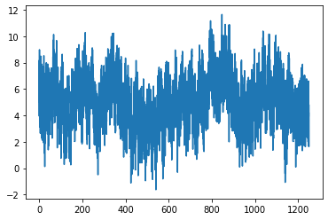
By passing a beta value as a function argument, the shape of power-law spectrum can be defined. Passing beta as 1 gives a flicker-noise distribution.
[5]:
lc = sim.simulate(1)
plt.errorbar(lc.time, lc.counts, yerr=lc.counts_err)
[5]:
<ErrorbarContainer object of 3 artists>
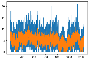
When simulating Poisson-distributed light curves, a smooth_counts attribute is added to the light curve, containing the original smooth light curve, for debugging purposes.
[6]:
lc_pois = sim_pois.simulate(1)
plt.plot(lc_pois.time, lc_pois.counts)
plt.plot(lc_pois.time, lc_pois.smooth_counts)
[6]:
[<matplotlib.lines.Line2D at 0x7fccd1d29c10>]
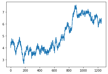
Passing beta as 2, gives random-walk distribution.
[7]:
lc = sim.simulate(2)

plt.errorbar(lc.time, lc.counts, yerr=lc.counts_err)
[7]:
<ErrorbarContainer object of 3 artists>
[8]:
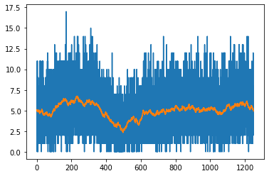
lc_pois = sim_pois.simulate(2)
plt.plot(lc_pois.time, lc_pois.counts)
plt.plot(lc_pois.time, lc_pois.smooth_counts)
[8]:
[<matplotlib.lines.Line2D at 0x7fccd3f9b9a0>]
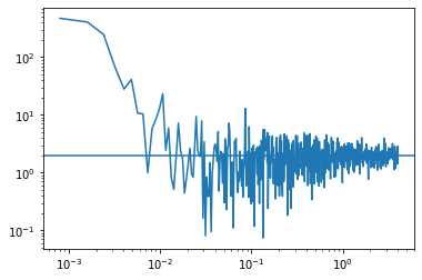
These light curves can be used for standard power spectral analysis with other Stingray classes.
[9]:
pds = Powerspectrum.from_lightcurve(lc_pois, norm="leahy")
pds = pds.rebin_log(0.005)
poisson = poisson_level(meanrate=lc_pois.meanrate, norm="leahy")
plt.loglog(pds.freq, pds.power)
plt.axhline(poisson)
[9]:
<matplotlib.lines.Line2D at 0x7fccd359b610>
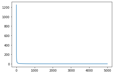
(ii) Using user-defined model
Light curve can also be simulated using a user-defined spectrum.
[10]:
w = np.fft.rfftfreq(sim.N, d=sim.dt)[1:]
spectrum = np.power((1/w),2/2)
plt.plot(spectrum)
[10]:
[<matplotlib.lines.Line2D at 0x7fccd5485b80>]
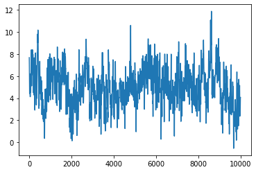
[11]:
lc = sim.simulate(spectrum)
plt.plot(lc.counts)
[11]:
[<matplotlib.lines.Line2D at 0x7fccd6506550>]
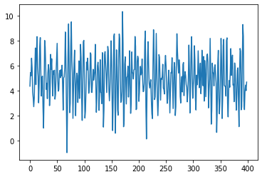
(iii) Using pre-defined models
One of the pre-defined spectrum models can also be used to simulate a light curve. In this case, model name and model parameters (as list iterable) need to be passed as function arguments.
To read more about the models and what the different parameters mean, see models notebook.
[12]:
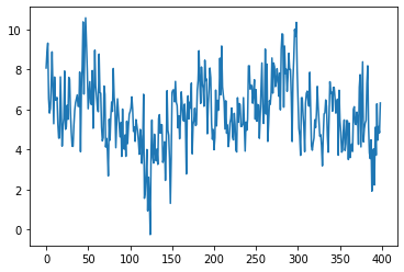
lc = sim.simulate('generalized_lorentzian', [1.5, .2, 1.2, 1.4])
plt.plot(lc.counts[1:400])
[12]:
[<matplotlib.lines.Line2D at 0x7fccb6d9b4f0>]
[13]:
lc = sim.simulate('smoothbknpo', [.6, 0.9, .2, 4])
plt.plot(lc.counts[1:400])
[13]:
[<matplotlib.lines.Line2D at 0x7fccb6dfddc0>]
(iv) Using impulse response
Before simulating a light curve through this approach, an appropriate impulse response needs to be constructed. There are two helper functions available for that purpose.
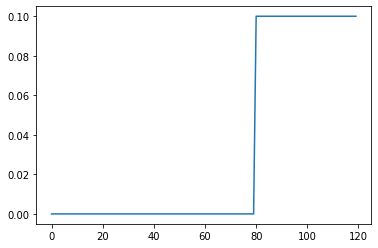
simple_ir() allows to define an impulse response of constant height. It takes in starting time, width and intensity as arguments, all of whom are set by default.
[14]:
s_ir = sim.simple_ir(10, 5, 0.1)
plt.plot(s_ir)
[14]:
[<matplotlib.lines.Line2D at 0x7fccd66015e0>]
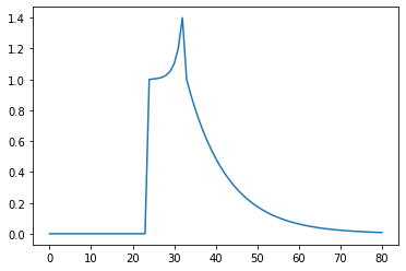
A more realistic impulse response mimicking black hole dynamics can be created using relativistic_ir(). Its arguments are: primary peak time, secondary peak time, end time, primary peak value, secondary peak value, rise slope and decay slope. These paramaters are set to appropriate values by default.
[15]:
r_ir = sim.relativistic_ir()
r_ir = sim.relativistic_ir(t1=3, t2=4, t3=10, p1=1, p2=1.4, rise=0.6, decay=0.1)
plt.plot(r_ir)
[15]:
[<matplotlib.lines.Line2D at 0x7fccd65955e0>]
Now, that the impulse response is ready, simulate() method can be called to produce a light curve.
[16]:
lc_new = sim.simulate(sample, r_ir)
Since, the new light curve is produced by the convolution of original light curve and impulse response, its length is truncated by default for ease of analysis. This can be changed, however, by supplying an additional parameter full.
[17]:
lc_new = sim.simulate(sample, r_ir, 'full')
Finally, some times, we do not need to include lag delay portion in the output light curve. This can be done by changing the final function parameter to filtered.
[18]:
lc_new = sim.simulate(sample, r_ir, 'filtered')
To learn more about what the lags look like in practice, head to the lag analysis notebook.
Channel Simulation
Here, we demonstrate simulator’s functionality to simulate light curves independently for each channel. This is useful, for example, when dealing with energy dependent impulse responses where you can create a new channel for each energy range and simulate.
In practical situations, different channels may have different impulse responses and hence, would react differently to incoming light curves. To account for this, there is an option to simulate light curves and add them to corresponding energy channels.
[19]:
sim.simulate_channel('3.5-4.5', 2)
sim.count_channels()
[19]:
1
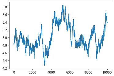
Above command assigns a light curve of random-walk distribution to energy channel of range 3.5-4.5. Notice, that simulate_channel() has the same parameters as simulate() with the exception of first parameter that describes the energy range of channel.
To get a light curve belonging to a specific channel, get_channel() is used.
[20]:
lc = sim.get_channel('3.5-4.5')
plt.plot(lc.counts)
[20]:
[<matplotlib.lines.Line2D at 0x7fccb763d340>]
A specific energy channel can also be deleted.
[21]:
sim.delete_channel('3.5-4.5')
sim.count_channels()
[21]:
0
Alternatively, if there are multiple channels that need to be added or deleted, this can be done by a single command.
[22]:
sim.simulate_channel('3.5-4.5', 1)
sim.simulate_channel('4.5-5.5', 'smoothbknpo', [.6, 0.9, .2, 4])
[23]:
sim.count_channels()
[23]:
2
[24]:
sim.get_channels(['3.5-4.5', '4.5-5.5'])
sim.delete_channels(['3.5-4.5', '4.5-5.5'])
[25]:
sim.count_channels()
[25]:
0
Reading/Writing
Simulator object can be saved or retrieved at any time using pickle.
[26]:
sim.write('data.pickle')
[27]:
sim.read('data.pickle')
[27]:
<stingray.simulator.simulator.Simulator at 0x7fccd6629640>