Contents

This notebook covers the pre-defined spectral models available for light curve simulation. Specifically, the notebook describes the meaning of different parameters that describe these models.

Setup

Import relevant stingray libraries.

from stingray.simulator import simulator, models

Import pyplot from matplotlib for plotting light curves.

from matplotlib import pyplot as plt
%matplotlib inline

Power Spectral Models

Currently, stingray has two spectral models namely generalized lorenzian function and smooth broken power law function. More models might be added in future, but, as explained in the rest of the section, Astropy models can be used to create most power spectral shapes one might be interested in.

Generalized Lorenzian Function

Apart from the frequencies, the lorenzian function needs the following parameters specified.

p: iterable
p[0] = peak centeral frequency
p[1] = FWHM of the peak (gamma)
p[2] = peak value at x=x0
p[3] = power coefficient [n]

Smooth Broken Power Law Model

Apart from the frequencies which need to be passed as a numpy array, smooth broken power law needs the following parameters specified.

p: iterable
p[0] = normalization frequency
p[1] = power law index for f --> zero
p[2] = power law index for f --> infinity
p[3] = break frequency

Light Curve Simulation

These models can be imported while simulating lightcurve(s).

sim = simulator.Simulator(N=1024, mean=0.5, dt=0.125, rms=0.2)

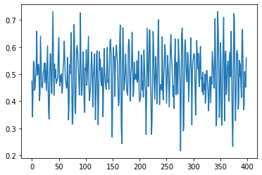
lc = sim.simulate('generalized_lorentzian', [1.5, .2, 1.2, 1.4])
plt.plot(lc.counts[1:400])

[<matplotlib.lines.Line2D at 0x7f86b4348910>]

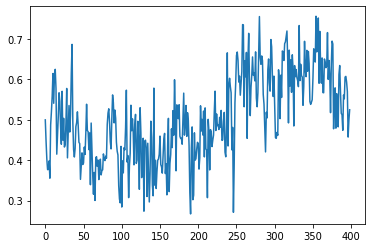
lc = sim.simulate('smoothbknpo', [.6, 0.9, .2, 4])
plt.plot(lc.counts[1:400])

[<matplotlib.lines.Line2D at 0x7f86b44f96a0>]