Lomb Scargle Cross Spectra
This tutorial shows how to make and manipulate a Lomb Scargle cross spectrum of two light curves using Stingray.
[1]:
from stingray.lightcurve import Lightcurve
from stingray.lombscargle import LombScargleCrossspectrum, LombScarglePowerspectrum
from scipy.interpolate import make_interp_spline
import numpy as np
import matplotlib.pyplot as plt
import matplotlib.font_manager as font_manager
plt.style.use('seaborn-v0_8-talk')
%matplotlib inline
from matplotlib.font_manager import FontProperties
font_prop = font_manager.FontProperties(size=16)
1. Create two light curves
There are two ways to make Lightcurve objects. We’ll show one way here. Check out Lightcurve for more examples.
Make two signals in units of counts. The first is a sine wave with random normal noise, frequency of 3 and at random times, and the second is another sine wave with frequency of 3, phase shift of 0.01/2pi and make their counts non-negative by subtracting its least value.
[2]:
rand = np.random.default_rng(42)
n = 100
t = np.sort(rand.random(n)) * 10
y = np.sin(2 * np.pi * 3.0 * t) + 0.1 * rand.standard_normal(n)
y2 = np.sin(2 * np.pi * 3.0 * (t+0.3)) + 0.1 * rand.standard_normal(n)
sub = min(np.min(y), np.min(y2))
y -= sub
y2 -= sub
Lets convert them into Lightcurve objects
[3]:
lc1 = Lightcurve(t, y)
lc2 = Lightcurve(t, y2)
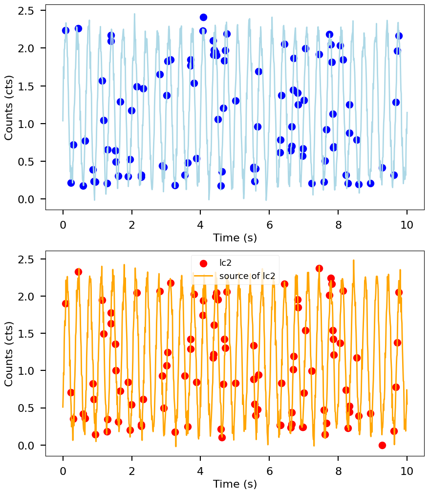
Let us plot them to see how they look
[4]:
t0 = np.linspace(0,10,1000)
y01 = np.sin(2 * np.pi * 3.0 * t0) + 0.1 * rand.standard_normal(t0.size)
y01 -= sub
y02 = np.sin(2 * np.pi * 3.0 * (t0+0.3)) + 0.1 * rand.standard_normal(t0.size)
y02 -= sub

spline1 = make_interp_spline(t0, y01)
spline2 = make_interp_spline(t0, y02)
t01 = np.linspace(0,10,1000)

fig, ax = plt.subplots(2,1,figsize=(10,12))
ax[0].scatter(lc1.time, lc1.counts, lw=2, color='blue',label='lc1')
ax[0].set_xlabel("Time (s)", fontproperties=font_prop)
ax[0].set_ylabel("Counts (cts)", fontproperties=font_prop)
ax[0].tick_params(axis='x', labelsize=16)
ax[0].tick_params(axis='y', labelsize=16)
ax[0].tick_params(which='major', width=1.5, length=7)
ax[0].tick_params(which='minor', width=1.5, length=4)
ax[0].plot(t01,spline1(t01),lw=2,color='lightblue',label='source of lc1')

ax[1].scatter(lc1.time, lc2.counts, lw=2, color='red',label='lc2')
ax[1].set_xlabel("Time (s)", fontproperties=font_prop)
ax[1].set_ylabel("Counts (cts)", fontproperties=font_prop)
ax[1].tick_params(axis='x', labelsize=16)
ax[1].tick_params(axis='y', labelsize=16)
ax[1].tick_params(which='major', width=1.5, length=7)
ax[1].tick_params(which='minor', width=1.5, length=4)
ax[1].plot(t01,spline2(t01),lw=2,color='orange',label='source of lc2')

plt.legend()
plt.show()
2. Pass both of the light curves to the LombScargleCrossspectrum class to create a LombScargleCrossspectrum object.
The first Lightcurve passed is the channel of interest or interest band, and the second Lightcurve passed is the reference band. You can also specify the optional attribute norm if you wish to normalize the real part of the cross spectrum to squared fractional rms, Leahy, or squared absolute normalization. The default normalization is ‘none’.
[5]:
lcs = LombScargleCrossspectrum(
    lc1,
    lc2,
    min_freq=0,
    max_freq=None,
    method="fast",
    power_type="all",
    norm="none",
)
We can print the first five values in the arrays of the positive Fourier frequencies and the power. The power has a real and an imaginary component.
[6]:
print(lcs.freq[0:5])
print(lcs.power[0:5])
[0.05163902 0.15491705 0.25819509 0.36147313 0.46475116]
[  6.31032111 +4.52192914j  63.18701964+17.6050907j
 118.96655765-28.2054288j   84.8747486 -42.95292067j
  -5.16601064+18.1110093j ]
Properties
Parameters
data1: This parameter allows you to provide the dataset for the first channel or band of interest. It can be either a`stingray.lightcurve.Lightcurve<https://docs.stingray.science/en/stable/core.html#working-with-lightcurves>`__ or`stingray.events.EventList<https://docs.stingray.science/en/stable/core.html#working-with-event-data>`__ object. It is optional, and the default value isNone.data2: Similar todata1, this parameter represents the dataset for the second channel or “reference” band. It follows the same format asdata1and is also optional with a default value ofNone.norm: This parameter defines the normalization of the cross spectrum. It takes string values from the set {frac,abs,leahy,none}. The default normalization is set tonone.power_type: This parameter allows you to specify the type of cross spectral power you want to compute. The options are:realfor the real part,absolutefor the magnitude, andallto compute both real part and magnitude. The default isall.fullspec: This is a boolean parameter that determines whether to keep only the positive frequencies or include both positive and negative frequencies in the cross spectrum. When set toFalse(default), only positive frequencies are kept; when set toTrue, both positive and negative frequencies are included.
Other Parameters
dt: When constructing light curves using`stingray.events.EventList<https://docs.stingray.science/en/stable/core.html#working-with-event-data>`__ objects, thedtparameter represents the time resolution of the light curve. It is a float value that needs to be provided.skip_checks: This is a boolean parameter that, when set toTrue, skips initial checks for speed or other reasons. It’s useful when you have confidence in the inputs and want to improve processing speed.min_freq: This parameter specifies the minimum frequency at which the Lomb-Scargle Fourier Transform should be computed.max_freq: Similarly, themax_freqparameter sets the maximum frequency for the Lomb-Scargle Fourier Transform.df: Thedfparameter, a float, represents the frequency resolution. It’s relevant when constructing light curves using`stingray.events.EventList<https://docs.stingray.science/en/stable/core.html#working-with-event-data>`__ objects.method: Themethodparameter determines the method used by the Lomb-Scargle Fourier Transformation function. The allowed values arefastandslow, with the default beingfast. Thefastmethod uses the optimized Press and Rybicki O(n*log(n)) algorithm.oversampling: This optional float parameter represents the interpolation oversampling factor. It is applicable when using the fast algorithm for the Lomb-Scargle Fourier Transform. The default value is 5.
Attributes
freq: Thefreqattribute is a numpy array that contains the mid-bin frequencies at which the Fourier transform samples the cross spectrum.power: Thepowerattribute is a numpy array that contains the complex numbers representing the cross spectra.power_err: Thepower_errattribute is a numpy array that provides the uncertainties associated with thepower. The uncertainties are approximated using the formulapower_err = power / sqrt(m), wheremis the number of power values averaged in each bin. For a single realization (m=1), the error is equal to the power.df: Thedfattribute is a float that indicates the frequency resolution.m: Themattribute is an integer representing the number of averaged cross-spectra amplitudes in each bin.n: Thenattribute is an integer indicating the number of data points or time bins in one segment of the light curves.k: Thekattribute is an array of integers indicating the rebinning scheme. If the object has been rebinned, the attribute holds the rebinning scheme; otherwise, it is set to 1.nphots1: Thenphots1attribute is a float representing the total number of photons in light curve 1.nphots2: Thenphots2attribute is a float representing the total number of photons in light curve 2.
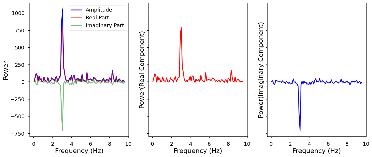
We can plot the cross spectrum by using the plot function or manually taking the freq and power attributes
[7]:
fig, ax = plt.subplots(1,3,figsize=(15,6),sharey=True)
lcs.plot(ax=ax[0])
ax[0].set_xlabel("Frequency (Hz)", fontproperties=font_prop)
ax[0].set_ylabel("Power", fontproperties=font_prop)
ax[1].plot(lcs.freq, lcs.power.real, lw=2, color='red')
ax[1].set_xlabel("Frequency (Hz)", fontproperties=font_prop)
ax[1].set_ylabel("Power(Real Component)", fontproperties=font_prop)
ax[2].plot(lcs.freq, lcs.power.imag, lw=2, color='blue')
ax[2].set_xlabel("Frequency (Hz)", fontproperties=font_prop)
ax[2].set_ylabel("Power(Imaginary Component)", fontproperties=font_prop)
[7]:
Text(0, 0.5, 'Power(Imaginary Component)')