Lomb Scargle Power Spectra

This tutorial shows how to make and manipulate a Lomb Scargle power spectrum of two light curves using Stingray.

from stingray.lightcurve import Lightcurve
from stingray.lombscargle import LombScarglePowerspectrum
import numpy as np
import matplotlib.pyplot as plt
from scipy.interpolate import make_interp_spline
import matplotlib.font_manager as font_manager
%matplotlib inline
plt.style.use('seaborn-v0_8-talk')
font_prop = font_manager.FontProperties(size=16)

1. Create a light curve

There are two ways to make Lightcurve objects. We’ll show one way here. Check out Lightcurve for more examples.

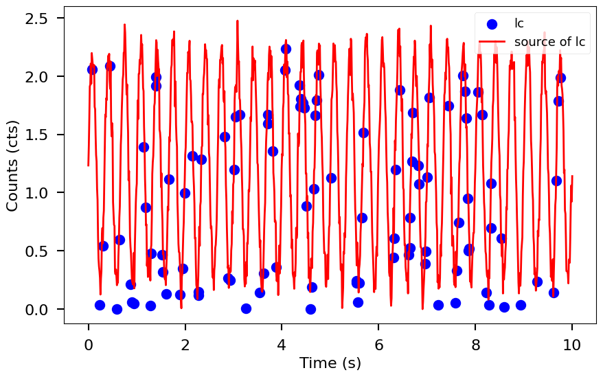
Make one with signals in units of counts. It is a sine wave with random normal noise, frequency of 3 and at random times and make its counts non-negative by subtracting its least value.

rand = np.random.default_rng(42)
n = 100
t = np.sort(rand.random(n)) * 10
y = np.sin(2 * np.pi * 3.0 * t) + 0.1 * rand.standard_normal(n)
sub = np.min(y)
y -= sub
t0 = np.linspace(0, 10, 1000)
y0 = np.sin(2 * np.pi * 3.0 * t0) + 0.1 * rand.standard_normal(t0.size)
sub = np.min(y0)
y0 -= sub
spline = make_interp_spline(t, y)

Lets convert them into Lightcurve objects

lc = Lightcurve(t, y)

Let us plot them to see how they look

fig, ax = plt.subplots(1,1,figsize=(10,6))
ax.scatter(lc.time, lc.counts, lw=2, color='blue',label='lc')
ax.plot(t0, y0, lw=2, color='red',label='source of lc')
ax.set_xlabel("Time (s)", fontproperties=font_prop)
ax.set_ylabel("Counts (cts)", fontproperties=font_prop)
ax.tick_params(axis='x', labelsize=16)
ax.tick_params(axis='y', labelsize=16)
ax.tick_params(which='major', width=1.5, length=7)
ax.tick_params(which='minor', width=1.5, length=4)
plt.legend()
plt.show()

2. Pass the light curve to the LombScarglePowerspectrum class to create a LombScarglePowerspectrum object.

You can also specify the optional attribute norm if you wish to normalize the real part of the power spectrum to squared fractional rms, Leahy, or squared absolute normalization. The default normalization is ‘none’.

lps = LombScarglePowerspectrum(
    lc,
    min_freq=0,
    max_freq=None,
    method="fast",
    power_type="all",
    norm="none",
)

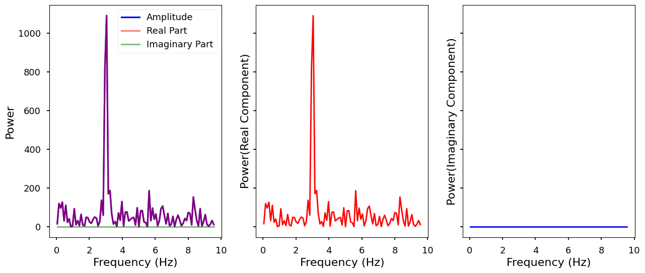
We can print the first five values in the arrays of the positive Fourier frequencies and the power. The power has only real component, and imaginary component is zero.

print(lps.freq[0:5])
print(lps.power[0:5])

[0.05163902 0.15491705 0.25819509 0.36147313 0.46475116]
[ 15.49526224+0.j 120.05686691+0.j  96.589673  +0.j 127.2231466 +0.j
  30.42053746+0.j]

Parameters

• data: This parameter allows you to provide the light curve data to be Fourier-transformed. It can be either a `stingray.lightcurve.Lightcurve <https://docs.stingray.science/en/stable/core.html#working-with-lightcurves>`__ or `stingray.events.EventList <https://docs.stingray.science/en/stable/core.html#working-with-event-data>`__ object. It is optional, and the default value is None.

• norm: The norm parameter defines the normalization of the power spectrum. It accepts string values from the set {frac, abs, leahy, none}. The default normalization is set to none.

• power_type: The power_type parameter allows you to specify the type of power spectral power you want to compute. The options are: real for the real part, absolute for the magnitude, and all to compute both real part and magnitude. The default is all.

• fullspec: This is a boolean parameter that determines whether to keep only the positive frequencies or include both positive and negative frequencies in the power spectrum. When set to False (default), only positive frequencies are kept; when set to True, both positive and negative frequencies are included.

Other Parameters

• dt: When constructing light curves using `stingray.events.EventList <https://docs.stingray.science/en/stable/core.html#working-with-event-data>`__ objects, the dt parameter represents the time resolution of the light curve. It is a float value that needs to be provided.

• skip_checks: This is a boolean parameter that, when set to True, skips initial checks for speed or other reasons. It’s useful when you have confidence in the inputs and want to improve processing speed.

• min_freq: This parameter specifies the minimum frequency at which the Lomb-Scargle Fourier Transform should be computed.

• max_freq: Similarly, the max_freq parameter sets the maximum frequency for the Lomb-Scargle Fourier Transform.

• df: The df parameter, a float, represents the frequency resolution. It’s relevant when constructing light curves using `stingray.events.EventList <https://docs.stingray.science/en/stable/core.html#working-with-event-data>`__ objects.

• method: The method parameter determines the method used by the Lomb-Scargle Fourier Transformation function. The allowed values are fast and slow, with the default being fast. The fast method uses the optimized Press and Rybicki O(n*log(n)) algorithm.

• oversampling: This optional float parameter represents the interpolation oversampling factor. It is applicable when using the fast algorithm for the Lomb-Scargle Fourier Transform. The default value is 5.

Attributes

• freq: The freq attribute is a numpy array that contains the mid-bin frequencies at which the Fourier transform samples the power spectrum.

• power: The power attribute is a numpy array that contains the normalized squared absolute values of Fourier amplitudes.

• power_err: The power_err attribute is a numpy array that provides the uncertainties associated with the power. The uncertainties are approximated using the formula power_err = power / sqrt(m), where m is the number of power values averaged in each bin. For a single realization (m=1), the error is equal to the power.

• df: The df attribute is a float that indicates the frequency resolution.

• m: The m attribute is an integer representing the number of averaged powers in each bin.

• n: The n attribute is an integer indicating the number of data points in the light curve.

• nphots: The nphots attribute is a float representing the total number of photons in the light curve.

We can plot the power spectrum by using the plot function or manually taking the freq and power attributes

fig, ax = plt.subplots(1,3,figsize=(15,6),sharey=True)
lps.plot(ax=ax[0])
ax[0].set_xlabel("Frequency (Hz)", fontproperties=font_prop)
ax[0].set_ylabel("Power", fontproperties=font_prop)
ax[1].plot(lps.freq, lps.power.real, lw=2, color='red')
ax[1].set_xlabel("Frequency (Hz)", fontproperties=font_prop)
ax[1].set_ylabel("Power(Real Component)", fontproperties=font_prop)
ax[2].plot(lps.freq, lps.power.imag, lw=2, color='blue')
ax[2].set_xlabel("Frequency (Hz)", fontproperties=font_prop)
ax[2].set_ylabel("Power(Imaginary Component)", fontproperties=font_prop)

Text(0, 0.5, 'Power(Imaginary Component)')