If clicking the link above turns the screen gray, try right clicking on the link and selecting “Open link in new tab”.

Install Stingray in colab

Comment out the cell below if running locally.

# %%capture --no-display
# !git clone --recursive https://github.com/StingraySoftware/stingray.git
# %cd stingray
# !pip install astropy scipy matplotlib numpy pytest pytest-astropy h5py tqdm seaborn
# !pip install -e "."
# %cd ..

# import os
# os.kill(os.getpid(), 9)

The kernel will (crash and then) restart after executing the above cell to finish installing Stingray. So the cells below will have to be run again or manually.

Multitaper Spectral Estimator Example

import numpy as np
import matplotlib.pyplot as plt
import seaborn as sns
sns.set_theme()
sns.set_palette("husl", 8)

import scipy
from scipy import signal
from stingray import Multitaper, Powerspectrum, Lightcurve

/home/dhruv/repos/stingray/stingray/largememory.py:25: UserWarning: Large Datasets may not be processed efficiently due to computational constraints
  warnings.warn(

### Creating a light curve

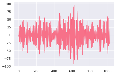
Lets create a Lightcurve sampled from an autoregressive process of order 4 that has been frequently exemplified in literature in similar contexts

np.random.seed(100)
coeff = np.array([2.7607, -3.8106, 2.6535, -0.9238]) # The 4 coefficients for the AR(4) process
ar4 = np.r_[1, -coeff] # For use with scipy.signal
N = 1024

freq_analytical, h = signal.freqz(b=1.0, a=ar4, worN=N, fs=1) # True PSD of AR(4)
psd_analytical = (h * h.conj()).real

data = signal.lfilter([1.0], ar4, np.random.normal(0, 1, N)) # N AR(4) data samples.

times = np.arange(N)

err = np.random.normal(0, 1, N)

lc_ar4 = Lightcurve(time=times, counts=data, err_dist='gauss', err=err)
lc_ar4.plot()

WARNING:root:Checking if light curve is well behaved. This can take time, so if you are sure it is already sorted, specify skip_checks=True at light curve creation.
WARNING:root:Checking if light curve is sorted.
/home/dhruv/repos/stingray/stingray/utils.py:126: UserWarning: SIMON says: Stingray only uses poisson err_dist at the moment. All analysis in the light curve will assume Poisson errors. Sorry for the inconvenience.
  warnings.warn("SIMON says: {0}".format(message), **kwargs)
WARNING:root:Computing the bin time ``dt``. This can take time. If you know the bin time, please specify it at light curve creation

The Multitaper Periodogram

Tapering a time series as a way of obtaining a spectral estimator with acceptable bias properties is an important concept. While tapering does reduce bias due to leakage, there is a price to pay in that the sample size is effectively reduced. The loss of information inherent in tapering can often be avoided either by prewhitening or by using Welch’s overlapped segment averaging.

The multitaper periodogram is another approach to recover information lost due to tapering. This apporach was introduced by Thomson (1982) and involves the use of multiple orthogonal tapers.

In the multitaper method the data is windowed or tapered, but this method differs from the traditional methods in the tapers used, which are the most band-limited functions amongst those defined on a finite time domain, and also, these tapers are orthogonal, enabling us to average the eigenspectrum (spectrum estimates from individual tapers) from more than one tapers to obtain a superior estimate in terms of noise. The resulting spectrum has low leakage, low variance, and retains information contained in the beginning and end of the time series. For more details on the multitaper periodogram, please have a look at the references.

Let’s have a look at the individual tapers.

NW = 4 # normalized half-bandwidth = 4
Kmax = 8 # Number of tapers
dpss_tapers, eigvals = \
signal.windows.dpss(M=lc_ar4.n, NW=NW, Kmax=Kmax,
                    sym=False, return_ratios=True)

data_multitaper = lc_ar4.counts - np.mean(lc_ar4.counts)  # De-mean
data_multitaper = np.tile(data_multitaper, (len(eigvals), 1))

 # Data tapered with the dpss windows
data_multitaper = np.multiply(data_multitaper, dpss_tapers)

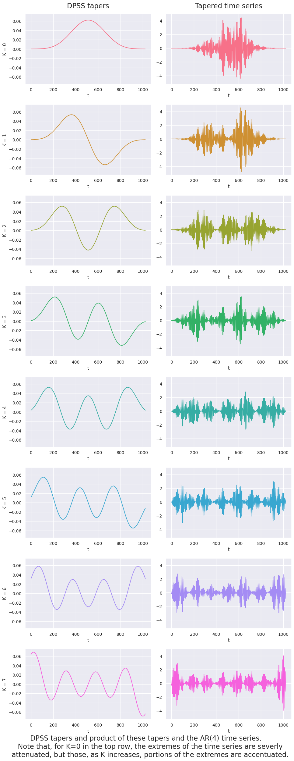
Plotted below are the first 8 tapers (on the left), and the corresponding tapered time series

fig, axes = plt.subplots(8, 2, figsize=(11, 27), dpi=90, sharey='col')

idx = 0
palette = sns.color_palette("husl", 8)
for taper, tapered_data, axes_rows in zip(dpss_tapers, data_multitaper, axes):
    axes_rows[0].plot(lc_ar4.time, taper, color=palette[idx])
    axes_rows[0].set_ylabel(f"K = {idx}")
    axes_rows[0].set_xlabel("t")

    axes_rows[1].plot(lc_ar4.time, tapered_data, color=palette[idx])
    axes_rows[1].set_xlabel("t")

    idx += 1
axes[0][0].set_title("DPSS tapers", fontsize=18, pad=15)
axes[0][1].set_title("Tapered time series", fontsize=18, pad=15)
fig.tight_layout()
txt="DPSS tapers and product of these tapers and the AR(4) time series.\n\
    Note that, for K=0 in the top row, the extremes of the time series are severly\n\
    attenuated, but those portions of the extremes, as K increases, are accentuated."
fig.text(.5, -0.025, txt, ha='center', fontsize=18)
fig.show();

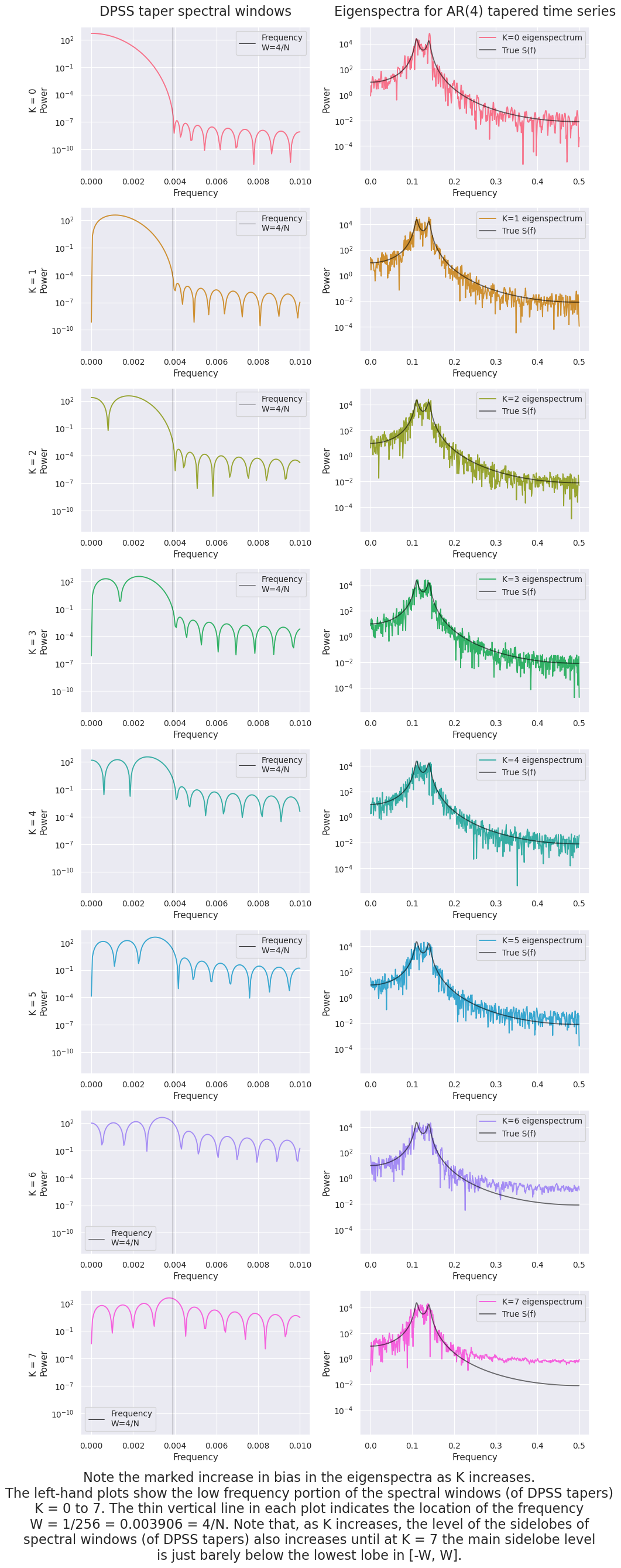
Now let’s see their frequency domain representations (here PSD)

We can have a good look at the leakage properties of these tapers (and the resulting time series) from their PSD representations.

%%capture --no-display
fig, axes = plt.subplots(8, 2, figsize=(11, 28), dpi=90, sharey='col')

idx = 0
palette = sns.color_palette("husl", 8)

freq = scipy.fft.rfftfreq(lc_ar4.n, d=lc_ar4.dt)
for taper, tapered_data, axes_rows in zip(dpss_tapers, data_multitaper, axes):

    w, h = signal.freqz(taper, fs=1, worN=np.linspace(0, 0.01, 200))
    h = np.multiply(h, np.conj(h))
    axes_rows[0].plot(w, h, color=palette[idx])
    axes_rows[0].axvline(x=NW/N, color="black", linewidth=0.6, label="Frequency\nW=4/N")
    axes_rows[0].set(
        ylabel=f"K = {idx} \nPower",
        xlabel="Frequency",
        yscale="log"
    )
    axes_rows[0].legend()

    fft_tapered_data = scipy.fft.rfft(tapered_data)
    psd_tapered_data = np.multiply(fft_tapered_data, np.conj(fft_tapered_data))
    axes_rows[1].plot(freq, psd_tapered_data, color=palette[idx], label=f"K={idx} eigenspectrum")
    axes_rows[1].plot(freq_analytical, psd_analytical, color="black", alpha=0.56, label="True S(f)")
    axes_rows[1].set(
        xlabel="Frequency",
        ylabel="Power",
        yscale="log"
    )
    axes_rows[1].legend()

    idx += 1
# fig.suptitle("Left: DPSS taper spectral windows \n Right: Eigenspectra for AR(4) time series with given K", y=1)
axes[0][0].set_title("DPSS taper spectral windows", fontsize=18, pad=15)
axes[0][1].set_title("Eigenspectra for AR(4) tapered time series", fontsize=18, pad=15)

text="Note the marked increase in bias in the eigenspectra as K increases.\n\
The left-hand plots show the low frequency portion of the spectral windows (of DPSS tapers)\n\
K = 0 to 7. The thin vertical line in each plot indicates the location of the frequency\n\
W = 1/256 = 0.003906 = 4/N. Note that, as K increases, the level of the sidelobes of\n\
spectral windows (of DPSS tapers) also increases until at K = 7 the main sidelobe level\n\
is just barely below the lowest lobe in [-W, W]."
fig.text(0.5, -0.06, text, ha="center", fontsize=18)
fig.tight_layout()
fig.show();

Summary of Multitaper Spectral Estimation

We assume that $ X_1, X_2, …, X_N $ is a sample of length \(N\) from a zero mean real-valued stationary process $ {X_t} $ with unknown sdf $ S(\cdot) $ defined over the interval \([-f_{(N)}, f_{(N)}]\), where \(f_{(N)} \equiv 1/(2\Delta t)\) is the Nyquist frequency and \(\Delta t\) is the sampling interval between observations. (If \(\{X_t\}\) has an unknown mean, we need to replace \(X_t\) with \(X_t' \equiv X_t - \bar{X_t}\) in all computational formulae, where \(\bar{X_t} = \sum^N_{t=1}X_t/N\) is the sample mean.)

• Simple multitaper spectral estimator \(\hat{S}^{mt}(\cdot)\)

This estimator is defined as the average of K eigenspectra \(\hat{S}^{mt}_k(\cdot),k = 0, ..., K - 1\), the \(k^{th}\) of which is a direct spectral estimator employing a dpss data taper \(\{h_{t,k}\}\) with parameter \(W\). The estimator \(\hat{S}^{mt}_k(f)\) is approximately equal in distribution to \(S(f)_{\chi^2_{2K}}/2K\)

• Adaptive multitaper spectral estimator \(\hat{S}^{amt}(\cdot)\)

This estimator uses the same eigenspectra as \(\hat{S}^{mt}(\cdot)\), but it now adaptively weights the \(\hat{S}^{mt}(\cdot)\) terms. The weight for the \(k^{th}\) eigenspectrum is proportional to \(b^2_k(f)\lambda_k\), where \(\lambda_k\) is the eigenvalue corresponding to the eigenvector with elements \(\{h_{t,k}\}\), while \(b_k(f)\) is given by

\(\large{b_k(f) = \frac {S(f)} {\lambda_k S(f) + (1-\lambda_k)\sigma^2\Delta t}}\)

The \(b_k(f)\) term depends on the unknown sdf \(S(f)\), but it is estimated using an iterative scheme. The estimator \(\hat{S}^{mt}_k(f)\) is approximately equal in distribution to \(S(f)_{\chi^2_\nu}/\nu\).

This summary, by no means, is an exhaustive explanation of the multitapering concept. Further exploration of the topic is highly encouraged. Use the references as the starting point.

Creating a Multitaper object

Pass the Lightcurve object to the Multitaper constructor ### Other (optional) parameters that can be set at instantiation are: (Given here for completness, feel free to skip as they are later showcased)

norm: {leahy | frac | abs | none }, optional, default frac

The normaliation of the power spectrum to be used. Options are leahy, frac, abs and none, default is frac.

NW: float, optional, default 4

The normalized half-bandwidth of the data tapers, indicating a multiple of the fundamental frequency of the DFT (Fs/N). Common choices are n/2, for n >= 4.

adaptive: boolean, optional, default False

Use an adaptive weighting routine to combine the PSD estimates of different tapers.

jackknife: boolean, optional, default True

Use the jackknife method to make an estimate of the PSD variance at each point.

low_bias: boolean, optional, default True

Rather than use 2NW tapers, only use the tapers that have better than 90% spectral concentration within the bandwidth (still using a maximum of 2NW tapers)

lombscargle: boolean, optional, default False

Whether to use the Lomb (1976) Scargle (1982) periodogram when calculating the Multitaper spectral estimate. Highly recommended for unevenly sampled time-series. Adaptive weighting and jack-knife estimated variance are yet not supported.

mtp = Multitaper(lc_ar4, adaptive=True, norm="abs")
print(mtp)

/home/dhruv/repos/stingray/stingray/utils.py:126: UserWarning: SIMON says: Stingray only uses poisson err_dist at the moment. All analysis in the light curve will assume Poisson errors. Sorry for the inconvenience.
  warnings.warn("SIMON says: {0}".format(message), **kwargs)

Using 7 DPSS windows for multitaper spectrum estimator
<stingray.multitaper.Multitaper object at 0x7fed1f89f130>

/home/dhruv/repos/stingray/stingray/utils.py:126: UserWarning: SIMON says: Looks like your lightcurve statistic is not poisson.The errors in the Powerspectrum will be incorrect.
  warnings.warn("SIMON says: {0}".format(message), **kwargs)

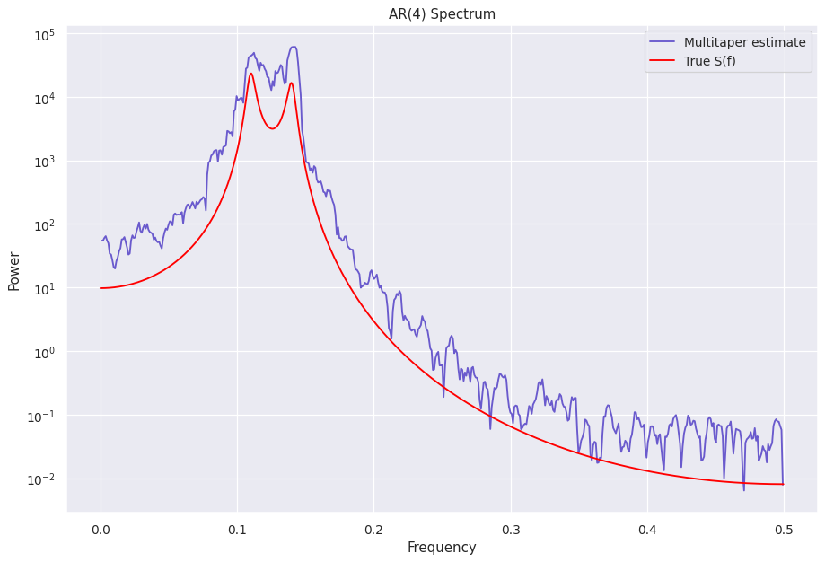
The results

fig = plt.figure(figsize=(12, 8), dpi=90)
plt.plot(mtp.freq, mtp.power, color="slateblue", label="Multitaper estimate")
plt.plot(freq_analytical, psd_analytical, color="red", label="True S(f)")
plt.yscale("log")
plt.legend()
plt.ylabel("Power")
plt.xlabel("Frequency")
plt.title("AR(4) Spectrum")
plt.show();

While it seems decent, lets compare with Powerspectrum

ps = Powerspectrum(lc_ar4, norm="abs")

/home/dhruv/repos/stingray/stingray/utils.py:126: UserWarning: SIMON says: Stingray only uses poisson err_dist at the moment. All analysis in the light curve will assume Poisson errors. Sorry for the inconvenience.
  warnings.warn("SIMON says: {0}".format(message), **kwargs)
/home/dhruv/repos/stingray/stingray/utils.py:126: UserWarning: SIMON says: Looks like your lightcurve statistic is not poisson.The errors in the Powerspectrum will be incorrect.
  warnings.warn("SIMON says: {0}".format(message), **kwargs)

fig = plt.figure(figsize=(12, 8), dpi=90)
plt.plot(mtp.freq, mtp.power, color="slateblue", label="Multitaper estimate")
plt.plot(ps.freq, ps.power, color="green", label="Periodogram estimate", alpha=0.4)
plt.plot(freq_analytical, psd_analytical, color="red", label="True S(f)")
plt.legend()
plt.yscale("log")
plt.ylabel("Power")
plt.xlabel("Frequency")
plt.title("AR(4) Spectrum")

Text(0.5, 1.0, 'AR(4) Spectrum')

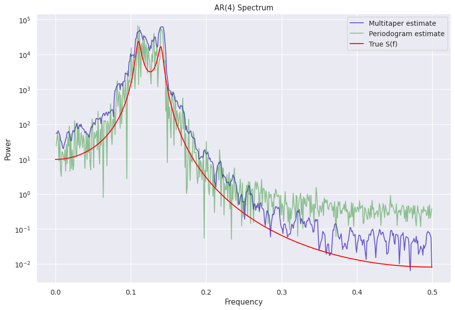
As can be seen, there is improvement in both the variance and the bias.

Attributes of the Multitaper object

norm: {leahy | frac | abs | none } the normalization of the power spectrun

freq: The array of mid-bin frequencies that the Fourier transform samples

power: The array of normalized squared absolute values of Fourier amplitudes

unnorm_power: The array of unnormalized values of Fourier amplitudes

multitaper_norm_power:The array of normalized values of Fourier amplitudes, normalized according to the scheme followed in nitime, that is, by the length and the sampling frequency.

power_err: The uncertainties of power. An approximation for each bin given by power_err = power/sqrt(m). Where m is the number of power averaged in each bin (by frequency binning, or averaging power spectrum). Note that for a single realization (m=1) the error is equal to the power.

df: The frequency resolution

m: The number of averaged powers in each bin

n: The number of data points in the light curve

nphots: The total number of photons in the light curve

jk_var_deg_freedom: Array differs depending on whether the jackknife was used. It is either - The jackknife estimated variance of the log-psd, OR - The degrees of freedom in a chi2 model of how the estimated PSD is distributed about the true log-PSD (this is either 2*floor(2*NW), or calculated from adaptive weights)

A look at the values contained in these attributes.

print(mtp)
print("norm: ", mtp.norm, type(mtp.norm))
print("power.shape: ", mtp.power.shape, type(mtp.power))
print("unnorm_power.shape: ", mtp.unnorm_power.shape, type(mtp.unnorm_power))
print("multitaper_norm_power.shape: ", mtp.multitaper_norm_power.shape, type(mtp.multitaper_norm_power))
print("power_err.shape: ", mtp.power_err.shape, type(mtp.power_err))
print("df: ", mtp.df, type(mtp.df))
print("m: ", mtp.m, type(mtp.m))
print("n: ", mtp.n, type(mtp.n)) # Notice the length of PSDs is half that of the number of data points in the light curve, as the imaginary (complex) part is discarded.
print("nphots: ", mtp.nphots, type(mtp.nphots))
print("jk_var_deg_freedom.shape: ", mtp.jk_var_deg_freedom.shape, type(mtp.jk_var_deg_freedom))

<stingray.multitaper.Multitaper object at 0x7fed1f89f130>
norm:  abs <class 'str'>
power.shape:  (511,) <class 'numpy.ndarray'>
unnorm_power.shape:  (511,) <class 'numpy.ndarray'>
multitaper_norm_power.shape:  (511,) <class 'numpy.ndarray'>
power_err.shape:  (511,) <class 'numpy.ndarray'>
df:  0.0009765625 <class 'numpy.float64'>
m:  1 <class 'int'>
n:  1024 <class 'int'>
nphots:  -73.38213649959974 <class 'numpy.float64'>
jk_var_deg_freedom.shape:  (511,) <class 'numpy.ndarray'>

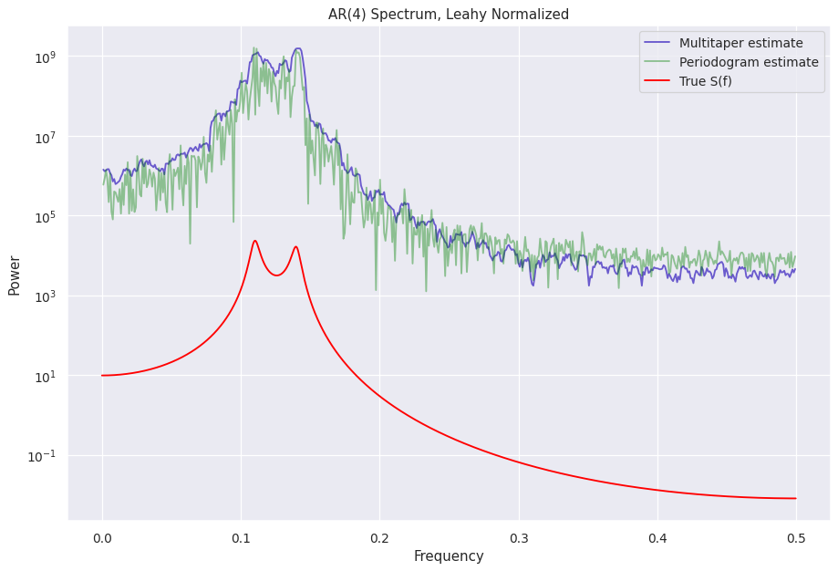
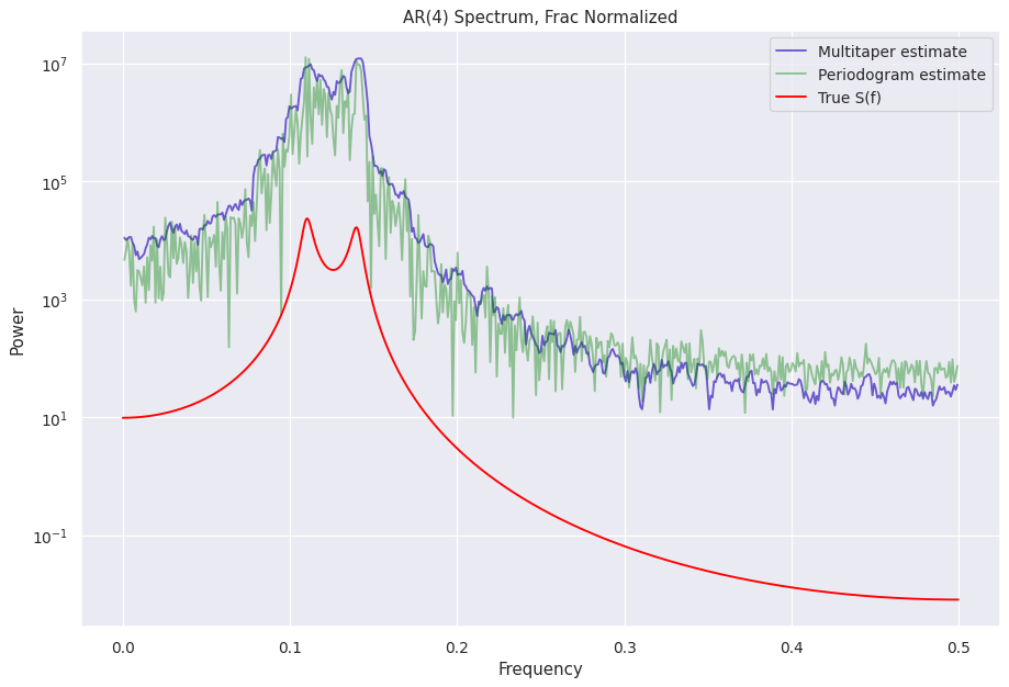
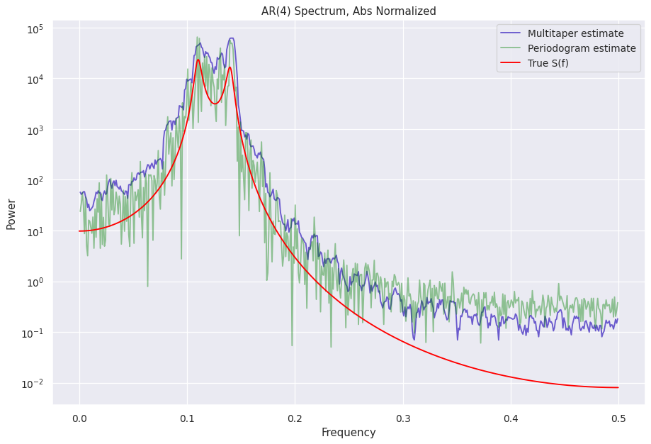
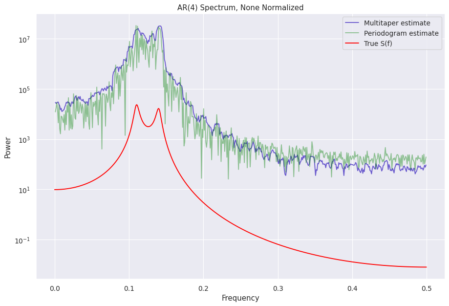
A look at the different normalizations

The normalized S(f) estimates are stored in the power attribute can be accessed like mtp.power if the object name is mtp

%%capture --no-display
norms = ["leahy", "frac", "abs", "none"]

for norm in norms:
    ps = Powerspectrum(lc_ar4, norm=norm)
    mtp = Multitaper(lc_ar4, norm=norm, adaptive=False) # adaptive=False does not calculate adaptive weights to reduce bias, helps see the normalization similarities better

    fig = plt.figure(figsize=(12, 8), dpi=90)
    plt.plot(mtp.freq, mtp.power, color="slateblue", label="Multitaper estimate")
    plt.plot(ps.freq, ps.power, color="green", label="Periodogram estimate", alpha=0.4)
    plt.plot(freq_analytical, psd_analytical, color="red", label="True S(f)")
    plt.legend()
    plt.yscale("log")
    plt.ylabel("Power")
    plt.xlabel("Frequency")
    plt.title("AR(4) Spectrum, " + (norm + " normalized").title())

Other attributes with the S(f) estimates

If you look closely at the attributes of the multitaper object, there is a multitaper_norm_power attribute. This attributes contains the PSD normalized according to

Another attribute containing the PSD is the unnorm_power, and as the name suggests, contains the unnormalized PSD.

A summary of the jackknife variance estimate

Assume that we have a sample of \(K\) independent observations, \(\{x_i\}, i = 1,...K\), drawn from some distribution characterized by a parameter \(\theta\), which is to be estimated. Here, \(\theta\) is usually a spectrum or coherence at a particular frequency or a simple parameter such as the frequency of a periodic component. Denote an estimate of \(\theta\) made using all \(K\) observations by \(\hat{\theta_{all}}\). Next, subdivide the data into \(K\) groups of size \(K − 1\) by deleting each entry in turn from the whole set, and let the estimate of \(\theta\) with the \(i\)th observation deleted be

\(\large{\theta_{\setminus i} = \hat{\theta}\{x_1,..x_{i-1},x_{i+1},...x_K\}}\)

for \(i = 1, 2,..., K\), where the subscript \(\setminus\) is the set-theoretic sense of without. Using \(\bullet\) in the statistical sense of averaged over, define the average of the \(K\) delete-one estimates as

\(\large{\theta_{\setminus \bullet} = \frac {1}{K} \sum_{i=1}^{K} \hat{ \theta_{\setminus i}}}\)

and the jackknife variance of \(\hat{\theta_{all}}\) as

\(\large{\widehat{Var}\{{\hat{\theta_{all}}}\} = \frac {K - 1}{K} \sum_{i=1}^{K} (\hat{ \theta_{\setminus i}}} - \hat{ \theta_{\setminus \bullet}})^2\)

This is just a summary of the jackknife variance estimate, kindly explore the references for further in-depth details.

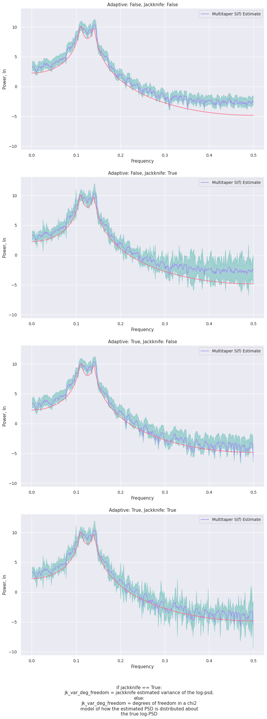
A look at jk_var_deg_freedom

This attribute differs depending on whether the jackknife was used. It is either - The jackknife estimated variance of the log-psd, OR - The degrees of freedom in a \(chi^2\) model of how the estimated PSD is distributed about the true log-PSD (this is either 2\(*\)floor(2\(*\)NW), or calculated from adaptive weights)

We’ll do a combination of the valid values for the adaptive and jk_var_deg_freedom and have a look at the results.

%%capture --no-display

# Setup utilities
import scipy.stats.distributions as dist

fig, axs = plt.subplots(4, 1, dpi=90, figsize=[11, 26], sharey=True)
fig.tight_layout(pad=4.0)

axs.flatten()
idx=0

for adaptive in (False, True):
    for jackknife in (False, True):

        mtp = Multitaper(lc_ar4, adaptive=adaptive, jackknife=jackknife)

        mtp_stingray = np.log(mtp.multitaper_norm_power)

        Kmax = len(mtp.eigvals)

        if jackknife:

            jk_p = (dist.t.ppf(.975, Kmax - 1) * np.sqrt(mtp.jk_var_deg_freedom))
            jk_limits_stingray = (mtp_stingray - jk_p, mtp_stingray + jk_p)

        else:

            p975 = dist.chi2.ppf(.975, mtp.jk_var_deg_freedom)
            p025 = dist.chi2.ppf(.025, mtp.jk_var_deg_freedom)

            l1 = np.log(mtp.jk_var_deg_freedom / p975)
            l2 = np.log(mtp.jk_var_deg_freedom / p025)

            jk_limits_stingray = (mtp_stingray + l1, mtp_stingray + l2)


        axs[idx].plot(mtp.freq, mtp_stingray, label="Multitaper S(f) Estimate", color=palette[6])
        axs[idx].fill_between(mtp.freq, jk_limits_stingray[0], y2=jk_limits_stingray[1], color=palette[4], alpha=0.4)

        axs[idx].plot(freq_analytical, np.log(psd_analytical), color=palette[0])

        axs[idx].set(
            title=f"Adaptive: {adaptive}, Jackknife: {jackknife}",
            ylabel="Power, ln",
            xlabel="Frequency"
        )
        axs[idx].legend()

        idx += 1


text = "if jackknife == True:\n\
jk_var_deg_freedom = jackknife estimated variance of the log-psd.\n\
else:\n\
jk_var_deg_freedom = degrees of freedom in a chi2\n\
model of how the estimated PSD is distributed about\n\
the true log-PSD"
fig.text(0.5, -0.05, text, ha="center")
fig.show();

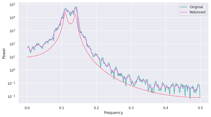
Linearly re-binning a power spectrum in frequency

mtp = Multitaper(lc_ar4, adaptive=True, norm="abs")
mtp_rebin = mtp.rebin(f=7)

print("Original df: ", mtp.df)
print("Rebinned df: ", mtp_rebin.df)

f = plt.figure(dpi=90, figsize=[11, 6])
plt.plot(mtp.freq, mtp.power, label="Original", color=palette[4])
plt.plot(mtp_rebin.freq, mtp_rebin.power, label="Rebinned", color=palette[7])
plt.plot(freq_analytical, psd_analytical, color=palette[0])
plt.legend()
plt.yscale("log")
plt.ylabel("Power")
plt.xlabel("Frequency")
f.show()

/home/dhruv/repos/stingray/stingray/utils.py:126: UserWarning: SIMON says: Stingray only uses poisson err_dist at the moment. All analysis in the light curve will assume Poisson errors. Sorry for the inconvenience.
  warnings.warn("SIMON says: {0}".format(message), **kwargs)
/home/dhruv/repos/stingray/stingray/utils.py:126: UserWarning: SIMON says: Looks like your lightcurve statistic is not poisson.The errors in the Powerspectrum will be incorrect.
  warnings.warn("SIMON says: {0}".format(message), **kwargs)

Using 7 DPSS windows for multitaper spectrum estimator
Original df:  0.0009765625
Rebinned df:  0.0068359375

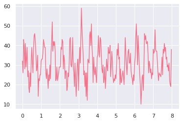
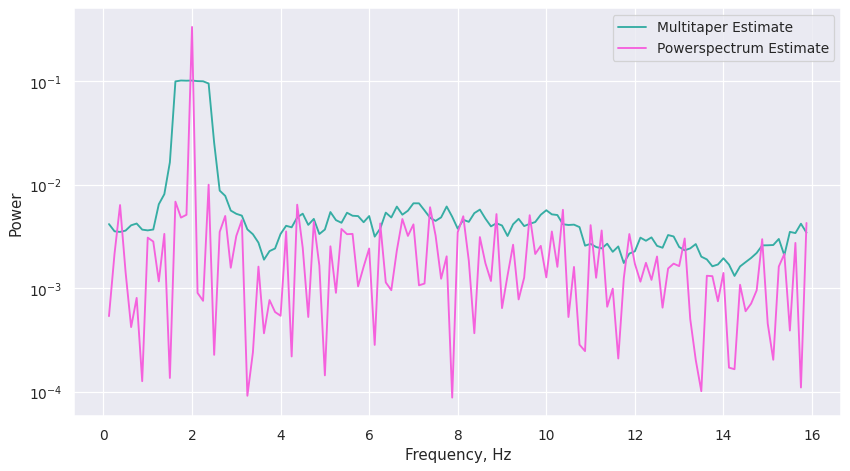
Poisson distributed lightcurve

Generate an array of relative timestamps that’s 8 seconds long, with dt = 0.03125 s, and make two signals in units of counts. The signal is a sine wave with amplitude = 300 cts/s, frequency = 2 Hz, phase offset = 0 radians, and mean = 1000 cts/s. We then add Poisson noise to the light curve.

dt = 0.03125  # seconds
exposure = 8.  # seconds
times = np.arange(0, exposure, dt)  # seconds

signal = 300 * np.sin(2.*np.pi*times/0.5) + 1000  # counts/s
noisy = np.random.poisson(signal*dt)  # counts

lc_poisson = Lightcurve(times, noisy, dt=dt)
lc_poisson.plot()

WARNING:root:Checking if light curve is well behaved. This can take time, so if you are sure it is already sorted, specify skip_checks=True at light curve creation.
WARNING:root:Checking if light curve is sorted.

Comparing Powerspectrum and Multitaper on poisson-distributed lightcurve

ps = Powerspectrum(lc_poisson)
mtp = Multitaper(lc_poisson, adaptive=True, low_bias=True)

f = plt.figure(dpi=90, figsize=[11, 6])
plt.plot(mtp.freq, mtp.power, label="Multitaper Estimate", color=palette[4])
plt.plot(ps.freq, ps.power, label="Powerspectrum Estimate", color=palette[7])
plt.legend()
plt.yscale("log")
plt.ylabel("Power")
plt.xlabel("Frequency, Hz")
f.show()

Using 7 DPSS windows for multitaper spectrum estimator

Time series with uneven temporal sampling: Multitaper Lomb-Scargle

Uneven temporal sampling is quite common in astronomical time series, and a popular method to deal with them is the Lomb-Scargle Periodogram.

A 2020 paper (A. Springford, et al.) used the Lomb-Scargle Periodogram in conjunction with the Multitapering concept for time-series with uneven sampling. That method is implemented here in Stingray.

Everthing works as before, just - Create a Lightcurve with the unevenly sampled time-series - Create a Multitaper object by passing it this Lightcurve object, with the desired value of NW, just additionally pass the ``lombscargle = True`` keyword during instantiation.

NOTE: Jack-knife variance estimation and adaptive weighting methods are not currently supported, so setting their keywords will have no effect if lombscargle = True.

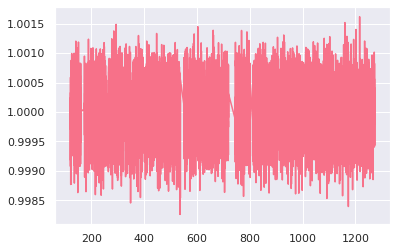
Testing the Multitaper Lomb-Scargle on a Kepler dataset (used in A. Springford et al. (2020) )

# Loading data
import pandas as pd

kepler_data = pd.read_csv("https://raw.githubusercontent.com/StingraySoftware/notebooks/tree/main/Multitaper/koi2133.csv")
times_kp = np.array(kepler_data["times"])
flux_kp = np.array(kepler_data["flux"])

lc_kepler = Lightcurve(time=times_kp, counts=flux_kp, err_dist="gauss", err=np.ones_like(times_kp))
lc_kepler.plot()

WARNING:root:Checking if light curve is well behaved. This can take time, so if you are sure it is already sorted, specify skip_checks=True at light curve creation.
WARNING:root:Checking if light curve is sorted.
/home/dhruv/repos/stingray/stingray/utils.py:126: UserWarning: SIMON says: Stingray only uses poisson err_dist at the moment. All analysis in the light curve will assume Poisson errors. Sorry for the inconvenience.
  warnings.warn("SIMON says: {0}".format(message), **kwargs)
WARNING:root:Computing the bin time ``dt``. This can take time. If you know the bin time, please specify it at light curve creation
/home/dhruv/repos/stingray/stingray/utils.py:126: UserWarning: SIMON says: Bin sizes in input time array aren't equal throughout! This could cause problems with Fourier transforms. Please make the input time evenly sampled.
  warnings.warn("SIMON says: {0}".format(message), **kwargs)

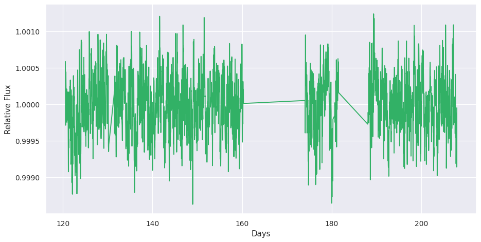
Plotting the first 3000 data points of the kepler lightcurve

The unevenness of the temporal sampling can be better seen with this

f = plt.figure(dpi=90, figsize=[12, 6])
plt.plot(lc_kepler.time[:3000], lc_kepler.counts[:3000], color=palette[3]);
plt.ylabel("Relative Flux")
plt.xlabel("Days")

Text(0.5, 0, 'Days')

%%time
mtls_kepler = Multitaper(lc_kepler, NW=10, lombscargle=True, norm="leahy") # Using normalized half bandwidth = 10

/home/dhruv/repos/stingray/stingray/utils.py:126: UserWarning: SIMON says: Stingray only uses poisson err_dist at the moment. All analysis in the light curve will assume Poisson errors. Sorry for the inconvenience.
  warnings.warn("SIMON says: {0}".format(message), **kwargs)

Using 19 DPSS windows for multitaper spectrum estimator
CPU times: user 19 s, sys: 4.61 s, total: 23.6 s
Wall time: 9.73 s

/home/dhruv/repos/stingray/stingray/utils.py:126: UserWarning: SIMON says: Looks like your lightcurve statistic is not poisson.The errors in the Powerspectrum will be incorrect.
  warnings.warn("SIMON says: {0}".format(message), **kwargs)

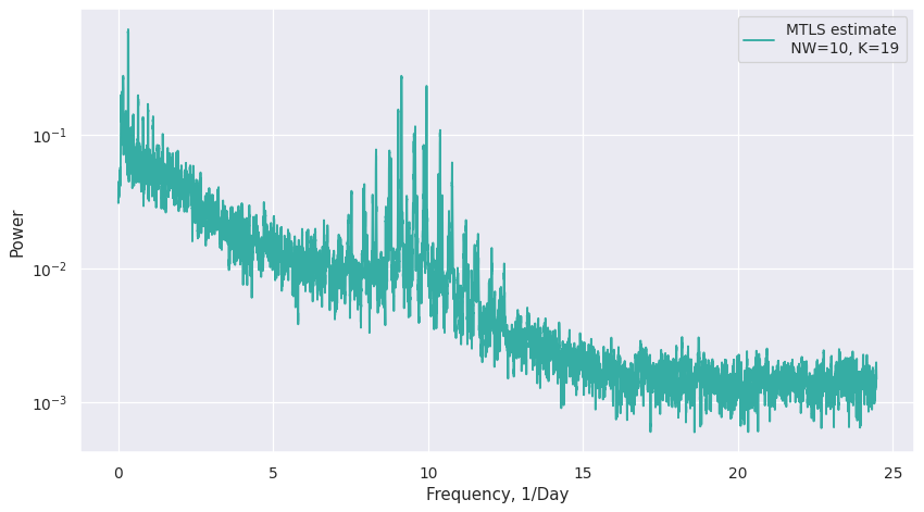
As stated before, the adaptive weighting method and jackknife log-psd estimate are currently not supported, hence these keywords will have no effect, no matter their value.

f = plt.figure(dpi=90, figsize=[11, 6])
plt.plot(mtls_kepler.freq, mtls_kepler.unnorm_power, label="MTLS estimate \n NW=10, K=19", color=palette[4])
plt.legend()
plt.yscale("log")
plt.ylabel("Power")
plt.xlabel("Frequency, 1/Day")
f.show()

But how does this compare to the classical Lomb-Scargle Periodogram?

from astropy.timeseries import LombScargle

ls_freq = scipy.fft.rfftfreq(n=lc_kepler.n, d=lc_kepler.dt)[1:-1] # Avioding zero
data =  lc_kepler.counts - np.mean(lc_kepler.counts)
ls_psd = LombScargle(lc_kepler.time, data).power(frequency=ls_freq, normalization="psd")

f, ax = plt.subplots(2, 1, dpi=90, figsize=[11, 11])
ax.flatten()
ax[0].plot(mtls_kepler.freq, mtls_kepler.power, label="MTLS estimate \n NW=10, K=19", color=palette[4])
ax[0].legend()
ax[0].set_yscale("log")
ax[0].set_ylabel("Power")
ax[0].set_xlabel("Frequency, 1/Day")

ax[1].plot(ls_freq, ls_psd, label="Lomb-Scargle Periodogram", color=palette[6])
ax[1].legend()
ax[1].set_ylabel("Power")
ax[1].set_yscale("log")
ax[1].set_xlabel("Frequency, 1/Day")
f.show()

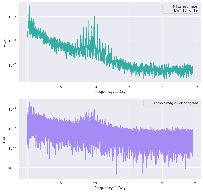
A pretty visual reduction in variance can be seen

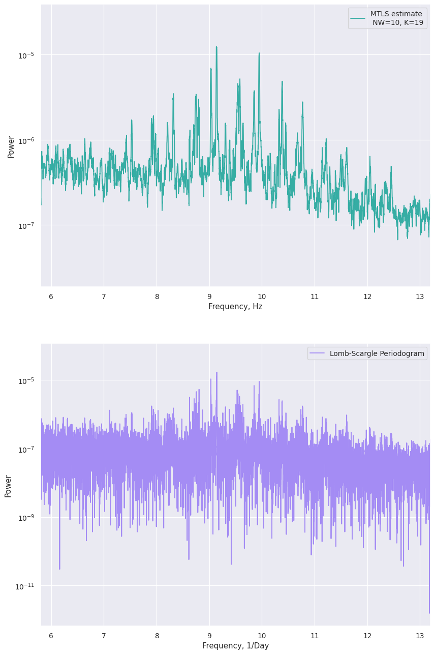
Zooming in

f, ax = plt.subplots(2, 1, dpi=90, figsize=[11, 18])
ax.flatten()
ax[0].plot(mtls_kepler.freq, mtls_kepler.power, label="MTLS estimate \n NW=10, K=19", color=palette[4])
ax[0].legend()
ax[0].set_ylabel("Power")
ax[0].set_xlabel("Frequency, Hz")
ax[0].set_yscale("log")
ax[0].set_xlim([5.8, 13.2])

ax[1].plot(ls_freq, ls_psd, label="Lomb-Scargle Periodogram", color=palette[6])
ax[1].legend()
ax[1].set_ylabel("Power")
ax[1].set_xlabel("Frequency, 1/Day")
ax[1].set_yscale("log")
ax[1].set_xlim([5.8, 13.2])
f.show()

References

[1] Springford, Aaron, Gwendolyn M. Eadie, and David J. Thomson. 2020. “Improving the Lomb–Scargle Periodogram with the Thomson Multitaper.” The Astronomical Journal (American Astronomical Society) 159: 205. doi:10.3847/1538-3881/ab7fa1.

[2] Huppenkothen, Daniela, Matteo Bachetti, Abigail L. Stevens, Simone Migliari, Paul Balm, Omar Hammad, Usman Mahmood Khan, et al. 2019. “Stingray: A Modern Python Library for Spectral Timing.” The Astrophysical Journal (American Astronomical Society) 881: 39. doi:10.3847/1538-4357/ab258d.

[3] Thomson, D. J. 1982. “Spectrum Estimation and Harmonic Analysis.” IEEE Proceedings 70: 1055-1096. https://ui.adsabs.harvard.edu/abs/1982IEEEP..70.1055T.

[4] Thomson, D. J. 1990 “Time series analysis of Holocene climate data.” Philosophical Transactions of the Royal Society of London. Series A, Mathematical and Physical Sciences (The Royal Society) 330: 601–616. doi:10.1098/rsta.1990.0041.

[5] Lomb, N. R. 1976. “Least-squares frequency analysis of unequally spaced data.” Astrophysics and Space Science (Springer Science and Business Media LLC) 39: 447–462. doi:10.1007/bf00648343.

[6] Scargle, J. D. 1982. “Studies in astronomical time series analysis. II - Statistical aspects of spectral analysis of unevenly spaced data.” The Astrophysical Journal (American Astronomical Society) 263: 835. doi:10.1086/160554.

[7] Slepian, D. 1978. “Prolate Spheroidal Wave Functions, Fourier Analysis, and Uncertainty-V: The Discrete Case.” Bell System Technical Journal (Institute of Electrical and Electronics Engineers (IEEE)) 57: 1371–1430. doi:10.1002/j.1538-7305.1978.tb02104.x.

[8] D. J. Thomson, “Jackknifing Multitaper Spectrum Estimates,” in IEEE Signal Processing Magazine, vol. 24, no. 4, pp. 20-30, July 2007, doi: 10.1109/MSP.2007.4286561.