Bispectrum Tutorial
This tutorial is intended to demonstrate bispectrum Analysis on Lightcurve data.
Bispectrum is an example of a Higher Order Spectra(HOS) and contains more information that simple Powerspectrum or non-ploy spectra. For detailed information on Bispectra visit : https://arxiv.org/pdf/1308.3150.pdf
In Stingray, Bispectrum can be created from a Lightcurve(For more information on Lightcurve, visit Lightcurve Notebook).
First we import relevant classes.
[2]:
from stingray import lightcurve
import numpy as np
from stingray.bispectrum import Bispectrum

import matplotlib.pyplot as plt
%matplotlib inline
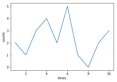
Lightcurve Object can be created from an array of time stamps and an array of counts. Creating a simple lightcurve to demonstrate Bispectrum.
[3]:
times = np.arange(1,11)
counts = np.array([2, 1, 3, 4, 2, 5, 1, 0, 2, 3])
lc = lightcurve.Lightcurve(times,counts)

lc.counts
[3]:
array([2, 1, 3, 4, 2, 5, 1, 0, 2, 3])
[4]:
lc.plot(labels=['times','counts'])
A Bispectrum Object takes 4 parameter.
lc: The light curve (lc).maxlag: Maximum lag on both positive and negative sides of 3rd order cumulant (Similar to lags in correlation).window: Specifies the type of window to apply as as stringscale: ‘biased’ or ‘unbiased’ for normalization
Arguments 2 and 3 are optional. If maxlag is not specified, it is set to no. of observations in lightcurve divided by 2. i.e lc.n/2 .
[5]:
bs = Bispectrum(lc)
Different attribute values can be observed by calling relevant properties. Most common are: 1. self.freq - Frequencies against which Bispectrum is calculated. 2. self.lags - Time lags in lightcurve against which 3rd order cumulant is calculated. 3. self.cum3 - 3rd Order cumulant function 4. self.bispec_mag - Magnitude of Bispectrum 5. self.bispecphase - Phase of Bispectrum
[6]:
bs.freq
[6]:
array([-0.5, -0.4, -0.3, -0.2, -0.1, 0. , 0.1, 0.2, 0.3, 0.4, 0.5])
[7]:
bs.lags
[7]:
array([-5., -4., -3., -2., -1., 0., 1., 2., 3., 4., 5.])
[8]:
bs.cum3
[8]:
array([[-0.3885, -0.0915,  0.1685, -0.5085,  0.8135, -0.0675, -0.2708,
         0.0229,  0.1426, -0.0567,  0.    ],
       [-0.0915,  0.2328, -0.5162, -2.0652,  0.3058,  0.1968,  0.8135,
         0.5492,  0.0209, -0.2484,  0.0063],
       [ 0.1685, -0.5162, -0.3999,  0.9821, -0.4989,  0.5011,  0.3058,
        -0.5085, -0.2348,  0.2379,  0.0426],
       [-0.5085, -2.0652,  0.9821, -0.3096,  0.5704,  2.1084, -0.4989,
        -2.0652,  0.1685,  0.8632,  0.0999],
       [ 0.8135,  0.3058, -0.4989,  0.5704, -1.3613, -0.3823,  0.5704,
         0.9821, -0.5162, -0.0915,  0.0872],
       [-0.0675,  0.1968,  0.5011,  2.1084, -0.3823,  0.864 , -1.3613,
        -0.3096, -0.3999,  0.2328, -0.3885],
       [-0.2708,  0.8135,  0.3058, -0.4989,  0.5704, -1.3613, -0.3823,
         0.5704,  0.9821, -0.5162, -0.0915],
       [ 0.0229,  0.5492, -0.5085, -2.0652,  0.9821, -0.3096,  0.5704,
         2.1084, -0.4989, -2.0652,  0.1685],
       [ 0.1426,  0.0209, -0.2348,  0.1685, -0.5162, -0.3999,  0.9821,
        -0.4989,  0.5011,  0.3058, -0.5085],
       [-0.0567, -0.2484,  0.2379,  0.8632, -0.0915,  0.2328, -0.5162,
        -2.0652,  0.3058,  0.1968,  0.8135],
       [ 0.    ,  0.0063,  0.0426,  0.0999,  0.0872, -0.3885, -0.0915,
         0.1685, -0.5085,  0.8135, -0.0675]])
[9]:
bs.bispec_mag
[9]:
array([[  6.1870122 ,   9.78649295,   6.29941723,   8.10990858,
          3.90975859,   1.49707597,  10.53408125,   8.44275685,
          7.73419771,   7.91909148,   3.40576093],
       [  9.78649295,  12.99063169,  11.9523207 ,  12.31681   ,
          7.34404789,   1.93438197,   5.05536311,  15.92827099,
          6.61153784,   3.09535492,   7.91909148],
       [  6.29941723,  11.9523207 ,   4.84009298,   8.98535468,
          5.6746004 ,   1.71227576,   9.35566037,  12.00797853,
          1.60576409,   6.61153784,   7.73419771],
       [  8.10990858,  12.31681   ,   8.98535468,  18.69373893,
          9.83780286,   2.72630968,   7.87985137,   5.32007463,
         12.00797853,  15.92827099,   8.44275685],
       [  3.90975859,   7.34404789,   5.6746004 ,   9.83780286,
          5.93123174,   1.60598497,   0.51743271,   7.87985137,
          9.35566037,   5.05536311,  10.53408125],
       [  1.49707597,   1.93438197,   1.71227576,   2.72630968,
          1.60598497,   1.262     ,   1.60598497,   2.72630968,
          1.71227576,   1.93438197,   1.49707597],
       [ 10.53408125,   5.05536311,   9.35566037,   7.87985137,
          0.51743271,   1.60598497,   5.93123174,   9.83780286,
          5.6746004 ,   7.34404789,   3.90975859],
       [  8.44275685,  15.92827099,  12.00797853,   5.32007463,
          7.87985137,   2.72630968,   9.83780286,  18.69373893,
          8.98535468,  12.31681   ,   8.10990858],
       [  7.73419771,   6.61153784,   1.60576409,  12.00797853,
          9.35566037,   1.71227576,   5.6746004 ,   8.98535468,
          4.84009298,  11.9523207 ,   6.29941723],
       [  7.91909148,   3.09535492,   6.61153784,  15.92827099,
          5.05536311,   1.93438197,   7.34404789,  12.31681   ,
         11.9523207 ,  12.99063169,   9.78649295],
       [  3.40576093,   7.91909148,   7.73419771,   8.44275685,
         10.53408125,   1.49707597,   3.90975859,   8.10990858,
          6.29941723,   9.78649295,   6.1870122 ]])
[10]:
bs.bispec_phase
[10]:
array([[ -7.65814471e-01,  -8.39758950e-01,   7.49083269e-01,
         -9.35797260e-01,  -1.22623935e+00,  -3.13514588e+00,
          4.35308043e-01,   6.65460441e-01,   6.17269495e-01,
          4.39881603e-01,  -3.14159265e+00],
       [ -8.39758950e-01,   1.84719564e+00,   1.70902436e+00,
         -6.50042861e-01,  -5.76818268e-01,  -9.16177187e-02,
          1.76512372e+00,   2.97853199e+00,   1.45401552e+00,
          0.00000000e+00,  -4.39881603e-01],
       [  7.49083269e-01,   1.70902436e+00,   1.64851065e+00,
         -5.51373516e-01,  -1.32816666e+00,   2.45429375e-01,
          2.86246989e+00,   3.08272440e+00,  -1.10623774e-15,
         -1.45401552e+00,  -6.17269495e-01],
       [ -9.35797260e-01,  -6.50042861e-01,  -5.51373516e-01,
         -2.97776986e+00,  -2.96295975e+00,  -4.83162811e-01,
          1.34000660e+00,   0.00000000e+00,  -3.08272440e+00,
         -2.97853199e+00,  -6.65460441e-01],
       [ -1.22623935e+00,  -5.76818268e-01,  -1.32816666e+00,
         -2.96295975e+00,  -1.30996608e+00,  -1.24358981e-01,
         -3.14159265e+00,  -1.34000660e+00,  -2.86246989e+00,
         -1.76512372e+00,  -4.35308043e-01],
       [ -3.13514588e+00,  -9.16177187e-02,   2.45429375e-01,
         -4.83162811e-01,  -1.24358981e-01,   3.14159265e+00,
          1.24358981e-01,   4.83162811e-01,  -2.45429375e-01,
          9.16177187e-02,   3.13514588e+00],
       [  4.35308043e-01,   1.76512372e+00,   2.86246989e+00,
          1.34000660e+00,   3.14159265e+00,   1.24358981e-01,
          1.30996608e+00,   2.96295975e+00,   1.32816666e+00,
          5.76818268e-01,   1.22623935e+00],
       [  6.65460441e-01,   2.97853199e+00,   3.08272440e+00,
          0.00000000e+00,  -1.34000660e+00,   4.83162811e-01,
          2.96295975e+00,   2.97776986e+00,   5.51373516e-01,
          6.50042861e-01,   9.35797260e-01],
       [  6.17269495e-01,   1.45401552e+00,   1.10623774e-15,
         -3.08272440e+00,  -2.86246989e+00,  -2.45429375e-01,
          1.32816666e+00,   5.51373516e-01,  -1.64851065e+00,
         -1.70902436e+00,  -7.49083269e-01],
       [  4.39881603e-01,   0.00000000e+00,  -1.45401552e+00,
         -2.97853199e+00,  -1.76512372e+00,   9.16177187e-02,
          5.76818268e-01,   6.50042861e-01,  -1.70902436e+00,
         -1.84719564e+00,   8.39758950e-01],
       [  3.14159265e+00,  -4.39881603e-01,  -6.17269495e-01,
         -6.65460441e-01,  -4.35308043e-01,   3.13514588e+00,
          1.22623935e+00,   9.35797260e-01,  -7.49083269e-01,
          8.39758950e-01,   7.65814471e-01]])
Plots
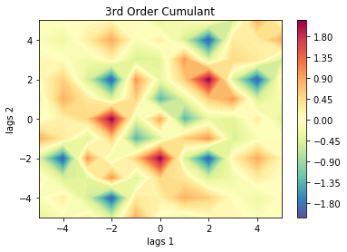
Bispectrum in stingray also provides functionality for contour plots of:
3rd Order Cumulant function
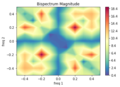
Magnitude Bispectrum
Phase Bispectrum
[11]:
p = bs.plot_cum3()
p.show()
[12]:
p = bs.plot_mag()
p.show()
[13]:
p = bs.plot_phase()
p.show()
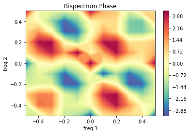
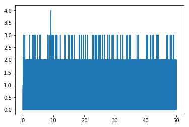
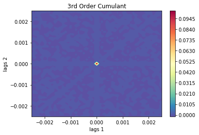
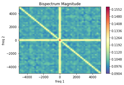
Another Example
Another example is demostrated here for a periodic lighturve with poisson noise.
[14]:
dt = 0.0001  # seconds
freq = 1 #Hz
exposure = 50.  # seconds
times = np.arange(0, exposure, dt)  # seconds

signal = 300 * np.sin(2.*np.pi*freq*times/0.5) + 1000  # counts/s
noisy = np.random.poisson(signal*dt)  # counts

lc = lightcurve.Lightcurve(times,noisy)
[15]:
lc.n
[15]:
500000
[16]:
lc.plot()
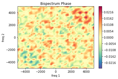
In this example, ‘unbiased’ scaled Bispectrum is calculated.
[17]:
bs = Bispectrum(lc, maxlag=25, scale='unbiased')
[18]:
bs.freq[:5]
[18]:
array([-5000.00000001, -4800.00000001, -4600.00000001, -4400.00000001,
       -4200.00000001])
[19]:
bs.lags[-5:]
[19]:
array([ 0.0021, 0.0022, 0.0023, 0.0024, 0.0025])
[20]:
bs.n
[20]:
500000
[21]:
bs.cum3[0]
[21]:
array([  4.16469688e-04,  -1.15175317e-06,  -1.07527932e-05,
         3.12465067e-05,  -1.49891250e-05,  -1.13491830e-05,
        -3.01378025e-05,   8.84909091e-06,  -9.76499980e-06,
        -4.03093430e-05,  -1.39169834e-05,  -1.06733571e-05,
        -3.56900080e-05,  -4.36904080e-05,  -1.64739272e-05,
        -6.07642325e-06,  -9.40724231e-05,   3.20972054e-05,
         1.10825598e-06,   1.57445478e-05,   1.50738698e-04,
        -1.53088049e-05,  -1.06758132e-05,  -8.50761732e-05,
        -2.70732731e-05,   5.15575763e-04,  -2.26276548e-06,
        -5.46966498e-05,  -3.49049233e-05,   6.93111630e-05,
        -1.96629892e-05,  -4.00897434e-05,  -5.37940654e-07,
        -1.25908665e-04,  -4.04722751e-05,  -1.95122973e-05,
         7.48985545e-06,  -1.59418559e-05,  -3.40950546e-07,
        -5.28946188e-05,  -6.77547458e-05,  -2.58282563e-06,
        -2.16597857e-05,   2.08264564e-05,   1.62145798e-05,
         6.20770115e-05,   5.74011370e-05,   3.04301082e-05,
         5.42455829e-05,   6.16520488e-05,   5.25699675e-05])
[22]:
bs.bispec_mag[1]
[22]:
array([ 0.10270301,  0.09674684,  0.1026435 ,  0.10278492,  0.09607422,
        0.09961388,  0.10090391,  0.10316149,  0.09881147,  0.10027435,
        0.09052907,  0.10086312,  0.09964639,  0.09224589,  0.10189853,
        0.09783874,  0.1029246 ,  0.10003251,  0.1003841 ,  0.09654483,
        0.10021589,  0.10265071,  0.09913028,  0.10406698,  0.10248613,
        0.12079938,  0.10038381,  0.09376602,  0.09916139,  0.10218425,
        0.09798569,  0.10296954,  0.10377357,  0.10144925,  0.09848511,
        0.09731673,  0.10031293,  0.09733791,  0.10085873,  0.09769191,
        0.10021328,  0.1000008 ,  0.10362033,  0.10352851,  0.09763424,
        0.10249754,  0.09752426,  0.09520164,  0.09959243,  0.12395456,
        0.10188173])
[23]:
bs.bispec_phase[1]
[23]:
array([ -1.44942123e-02,   1.67988284e-02,  -3.06544878e-03,
         1.24304742e-02,  -4.69267453e-04,   1.80410887e-02,
         1.18875941e-03,  -1.85154750e-03,   2.17338081e-02,
         1.03821918e-02,  -7.09489717e-03,   1.05358508e-02,
         4.01625879e-03,  -2.05403388e-02,   1.17686452e-03,
         2.56746832e-02,   2.17353559e-02,  -7.69020683e-03,
         1.54447950e-02,  -9.03814639e-04,   3.43660863e-03,
        -5.37971533e-04,   9.42017522e-03,   1.42720920e-03,
         1.17025084e-03,  -5.00982277e-03,  -1.53439701e-02,
        -7.63874625e-04,  -4.10637611e-02,   2.41131565e-02,
        -1.95500843e-02,  -2.98681684e-02,   1.23914953e-03,
        -2.75100800e-02,  -3.88428578e-03,  -7.87537903e-03,
        -1.53613857e-03,   1.47624077e-02,  -4.86162981e-03,
        -2.76731089e-03,   9.30828311e-03,  -2.86531767e-02,
        -1.16465064e-02,  -2.30165990e-02,  -7.71187242e-03,
         2.00694116e-02,  -5.16511843e-02,  -1.98737477e-03,
        -9.87738671e-03,  -2.09922507e-17,   1.39146079e-02])
[24]:
p = bs.plot_cum3()
p.show()
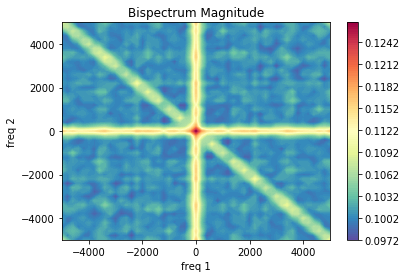
[25]:
p = bs.plot_mag()
p.show()
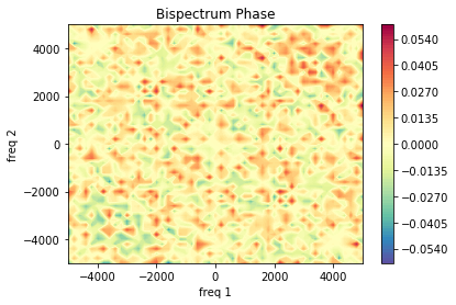
[26]:
p = bs.plot_phase()
p.show()
Window Functions for Bispectrum
Bispectrum in Stingray now supports 2D windows to apply before calculating Bispectrum.
Windows currently available in Stingray include: 1. Uniform or Rectangular window 2. Parzen Window 3. Hamming Window 4. Hanning Window 5. Triangular Window 6. Blackmann’s Window 7. Welch Window 8. Flat-top Window
Windows are available in stingray.utils package and can be used by calling create_window function.
Now, we demonstrate Bispectrum with windows applied. By default, now window is applied.
[29]:
window = 'uniform'

bs = Bispectrum(lc,maxlag=25,window = window, scale ='unbiased')
[30]:
bs.window_name
[30]:
'uniform'
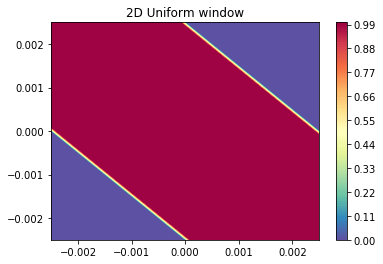
Plot Window
[32]:
cont = plt.contourf(bs.lags, bs.lags, bs.window, 100, cmap=plt.cm.Spectral_r)
plt.colorbar(cont)
plt.title('2D Uniform window')
[32]:
<matplotlib.text.Text at 0x1ac8b7e8e80>
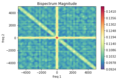
[34]:
mag_plot = bs.plot_mag()
mag_plot.show()
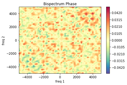
[35]:
phase_plot = bs.plot_phase()
phase_plot.show()
Now, let us try some more window functions.
[36]:
bs = Bispectrum(lc, maxlag=25,window = 'hamming',scale='biased')
[37]:
bs.window_name
[37]:
'hamming'
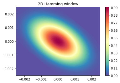
[38]:
cont = plt.contourf(bs.lags, bs.lags, bs.window, 100, cmap=plt.cm.Spectral_r)
plt.colorbar(cont)
plt.title('2D Hamming window')
[38]:
<matplotlib.text.Text at 0x1ac8bbfe710>
[39]:
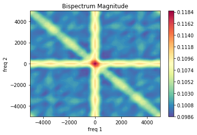
mag_plot = bs.plot_mag()
mag_plot.show()
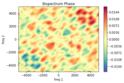
[40]:
phase_plot = bs.plot_phase()
phase_plot.show()
Another Window demonstrated
[45]:
bs = Bispectrum(lc, maxlag = 25, window='triangular',scale='unbiased')
[46]:
bs.window_name
[46]:
'triangular'
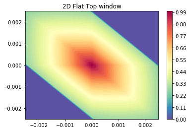
[47]:
cont = plt.contourf(bs.lags, bs.lags, bs.window, 100, cmap=plt.cm.Spectral_r)
plt.colorbar(cont)
plt.title('2D Flat Top window')
[47]:
<matplotlib.text.Text at 0x1ac8bdc15f8>
[48]:
bs.plot_mag().show()
[52]:
bs.plot_phase().show()