Start here to begin with Stingray.
[1]:
%load_ext autoreload
%autoreload 2

import numpy as np
%matplotlib inline
import warnings
warnings.filterwarnings('ignore')
Introduction
StingrayTimeseries is a generic time series object, and also acts as the base class for Stingray’s Lightcurve and EventList. It is a data container that associate times with measurements. The only compulsory element in such a series is indeed the time attribute.
Many of the methods in Lightcurve and EventList, indeed, are implemented in this class. For example, methods that truncate, add, subtract the series, or that filter it in some way (e.g. by adding a mask or applying the good time intervals)
Internal Class structure
For most of this internal behavior, all turns around the concept of “Array attributes”, “Internal attributes”, “Meta attributes”, and “Not array attributes”.
Array attributes Ideally, if one were to create a new object based on a table format, array attributes would be the table columns (so, they all have the same length of the time column). Example array attributes are
counts, the number of counts in each bin of a typical X-ray light curve;dt, the sampling time, if data are not evenly sampled;
Note that array attributes can have any dimension. The only important thing is that the first dimension’s size is equal to the size of time. E.g. if time is [1, 2, 3] (shape (3,) ), an array attribute could be [[4, 4], [2, 3], [4, 5]] (shape (3, 2)), but not [[1, 2, 3]] (shape (1, 3))
Meta attributes The most useful attributes are probably
gti, or the Good Time Intervals where measurements are supposed to be reliable;dt, the sampling time, when constant (evenly sampled time series);mjdrefthe reference MJD for all the time measurements in the series
Internal array attributes Some classes, like Lightcurve, expose attributes (such as counts, counts_err) that are not arrays but properties. This is done for a flexible manipulation of counts, count rates etc, that can be set asynchronously depending on which one was set first (see the Lightcurve documentation). The actual arrays containing data are internal attributes (such as _counts) that get set only if needed. Another thing that lightcurve does is throwing an error if
one wants to set the time to a different length than its array attributes. The actual time is stored in the _time attribute, and this check is done when one tries to modify the time through the time property (by setting lc.time).
Not array attributes Some quantities, such as GTI, might in principle have the same length of time. One can then add gti to the list of not_array_attributes, that protects from the hypothesis of considering gti a standard array attribute.
Creating a time series
[2]:
from stingray import StingrayTimeseries
A StingrayTimeseries object is usually created in one of the following two ways:
From an array of time stamps and an array of any name.
ts = StingrayTimeseries(times, array_attrs=dict(my_array_attr=my_attr), **opts)
where
**optsare any (optional) keyword arguments (e.g.dt=0.1,mjdref=55000, etc.) In principle, array attributes can be specified as simple keyword arguments. But when we use thearray_attrskeyword, we will run a check on the length of the arrays, and raise an error if they are not of a shape compatible with thetimearray.A binned
StingrayTimeseries, a generalization of a uniformly sampled light curve, can be obtained from an EventList object, through theto_binned_timeseriesmethod.ev = EventList(times, mjdref=55000) ev.my_attr = my_attr_array ts = ev.to_binned_timeseries(ev, dt=1, array_attrs={"my_attr": my_attr}, **opts)
as will be described in the next sections.
An additional possibility is creating an empty StingrayTimeseries object, whose attributes will be filled in later:
ts = StingrayTimeseries()
or, if one wants to specify any keyword arguments:
ts = StingrayTimeseries(**opts)
This option is usually only relevant to advanced users, but we mention it here for reference
1. Array of time stamps and counts
Create 1000 time stamps
[3]:
times = np.arange(1000)
times[:10]
[3]:
array([0, 1, 2, 3, 4, 5, 6, 7, 8, 9])
Create 1000 random Poisson-distributed counts:
[4]:
my_attr = np.random.normal(size=len(times))
my_attr[:10]
[4]:
array([ 0.24828431,  1.65343943,  0.48755812,  0.53731942,  0.06821194,
        0.67721999, -1.52268207,  0.90104872, -1.54513351,  0.4345529 ])
Create a Lightcurve object with the times and counts array.
[5]:
ts = StingrayTimeseries(times, array_attrs={"my_attr": my_attr})
The number of data points can be counted with the len function, or through the n property.
[6]:
len(ts), ts.n
[6]:
(1000, 1000)
2. From an event list
Often, you might have an event list with associated properties such as weight, polarization, etc. If this is the case, you can use the to_binned_timeseries method of EventList to turn these photon arrival times into a regularly binned timeseries.
[7]:
from stingray import EventList

arrival_times = np.sort(np.random.uniform(0, 100, 1000))
goofy = np.random.normal(size=arrival_times.size)
mickey = np.random.chisquare(2, size=arrival_times.size)
ev = EventList(arrival_times, gti=[[0, 100]])
ev.goofy = goofy
ev.mickey = mickey
To create the time series, it’s necessary to specify the sampling time dt. By default, the time series will create histograms with all the array attributes of EventLists with the same length as ev.time.
[8]:
ts_new = ev.to_binned_timeseries(dt=1)
One can specify which attributes to use through the array_attrs keyword
[9]:
ts_new_small = ev.to_binned_timeseries(dt=1, array_attrs=["goofy"])
All attributes that have been histogrammed can be accessed through the array_attrs method:
[10]:
ts_new.array_attrs()
[10]:
['counts', 'goofy', 'mickey']
[11]:
ts_new_small.array_attrs()
[11]:
['counts', 'goofy']
Note the counts attribute, which is always created by the to_binned_timeseries method and gives the number of photons which concurred to creating each value of the time series.
The time bins can be seen with the .time attribute
[12]:
ts_new.time
[12]:
array([ 0.5,  1.5,  2.5,  3.5,  4.5,  5.5,  6.5,  7.5,  8.5,  9.5, 10.5,
       11.5, 12.5, 13.5, 14.5, 15.5, 16.5, 17.5, 18.5, 19.5, 20.5, 21.5,
       22.5, 23.5, 24.5, 25.5, 26.5, 27.5, 28.5, 29.5, 30.5, 31.5, 32.5,
       33.5, 34.5, 35.5, 36.5, 37.5, 38.5, 39.5, 40.5, 41.5, 42.5, 43.5,
       44.5, 45.5, 46.5, 47.5, 48.5, 49.5, 50.5, 51.5, 52.5, 53.5, 54.5,
       55.5, 56.5, 57.5, 58.5, 59.5, 60.5, 61.5, 62.5, 63.5, 64.5, 65.5,
       66.5, 67.5, 68.5, 69.5, 70.5, 71.5, 72.5, 73.5, 74.5, 75.5, 76.5,
       77.5, 78.5, 79.5, 80.5, 81.5, 82.5, 83.5, 84.5, 85.5, 86.5, 87.5,
       88.5, 89.5, 90.5, 91.5, 92.5, 93.5, 94.5, 95.5, 96.5, 97.5, 98.5,
       99.5])
Good Time Intervals
StingrayTimeseries (and most other core stingray classes) support the use of Good Time Intervals (or GTIs), which denote the parts of an observation that are reliable for scientific purposes. Often, GTIs introduce gaps (e.g. where the instrument was off, or affected by solar flares). By default. GTIs are passed and don’t apply to the data within a StingrayTimeseries object, but become relevant in a number of circumstances, such as when generating Powerspectrum objects.
If no GTIs are given at instantiation of the StingrayTimeseries class, an artificial GTI will be created spanning the entire length of the data set being passed in, including half a sample time before and after:
[13]:
times = np.arange(1000)
counts = np.random.poisson(100, size=len(times))

ts = StingrayTimeseries(times, array_attrs={"counts":counts}, dt=1)
[14]:
ts.gti
[14]:
array([[-5.000e-01, 9.995e+02]])
[15]:
ts.counts
[15]:
array([ 96,  92,  92, 103, 101,  95, 112, 108,  97,  92, 102,  88,  82,
        82,  98, 107,  94,  90, 116,  97, 104, 109, 103,  90,  98, 104,
        91, 103,  89, 103, 116,  88,  96, 106, 106,  81,  92,  99,  88,
        88, 114,  95,  84, 102,  99,  89,  97,  84,  88, 100, 100,  89,
        86, 100, 100, 110, 106,  95, 117, 113, 101,  99,  95,  97, 108,
       107, 112,  82, 122, 101,  98,  94, 106, 109,  96, 103, 125, 105,
       107,  95,  91,  94,  92, 118,  90, 101,  96, 113,  95, 109,  92,
       101, 101,  97, 107, 109, 110, 113, 100, 113, 110,  91,  99, 103,
        98,  94,  99,  99,  87,  92,  96, 111, 105,  91,  88,  83, 107,
        78, 102,  90,  99,  96,  99, 107,  90, 111,  86, 129, 105,  98,
        91, 100, 118,  95,  97, 106,  96, 117, 107, 102, 101,  98,  89,
       105, 104, 104,  85, 113,  89,  89, 117, 111, 112, 117, 102, 129,
       105,  99, 106,  83,  83,  93, 114,  91, 116,  90, 117, 109,  95,
       103, 102,  90,  95,  83,  99, 108,  80, 104, 111, 107, 100,  87,
        87,  97, 100, 115, 107,  93, 106,  76, 105,  88, 100,  99,  99,
        89,  87,  89, 105, 106,  88, 113,  95, 120,  96, 107,  96, 114,
        97, 106, 106,  94,  83, 111,  91, 109,  93, 108, 106, 100,  85,
        84, 107, 126, 102,  99,  95, 100, 103,  90,  92,  89,  84, 120,
       114,  98, 117,  97, 109,  95, 100,  97,  84,  90, 110, 103, 108,
        92,  82, 115, 115,  97, 121, 104,  98,  89,  80,  99,  86,  98,
        97, 100,  96,  96, 125, 112,  95,  86,  94, 100,  91, 123,  98,
        76,  84, 109,  87,  92, 108,  89,  94,  94, 101, 110,  94,  94,
       106, 103,  99, 117,  87, 101,  97,  79, 117, 107, 111, 113, 107,
       106, 109, 104, 102,  99, 114,  89, 109,  95, 111,  75,  99, 115,
        91, 118, 112,  91,  87, 106,  94,  98, 102, 110,  92,  84,  97,
       118, 108,  89,  98,  99, 109, 122, 105, 101, 102, 107, 120,  87,
        90, 109, 100, 107, 107,  98,  96,  90, 100, 115,  92,  86, 100,
       114, 109,  91,  98,  96,  91, 105,  95,  93,  86,  85, 109, 107,
        97, 101, 101, 119,  98, 111, 102, 101, 107, 107,  89, 107,  93,
        98,  91, 102,  91, 116, 105,  98, 105,  95, 106,  99, 122, 111,
       108,  84, 100, 111,  91,  86,  95, 104,  95, 129, 103,  80,  90,
       105, 112,  97, 107, 113, 103,  96, 100,  99, 101, 111,  81, 110,
       101,  97,  98, 108,  96,  97,  95, 107,  91,  89, 108,  99,  85,
        97,  86, 103,  94, 111,  94,  83,  99,  91, 103,  96,  99,  98,
        94, 111, 101,  93,  88,  98, 105,  88, 125, 109, 107, 100,  95,
       104,  87,  97, 110,  98,  85, 114,  96, 116, 115,  99,  86,  96,
       101,  99,  84,  96,  96, 104,  85,  86,  98, 109, 102,  90, 111,
       104,  92, 107, 103, 101,  91, 106, 105,  93,  99, 108, 110,  85,
        88,  93, 105, 105, 120,  87, 103, 101, 125,  81,  94,  89, 107,
        96, 103, 104,  98,  98,  88, 108,  79,  92, 113, 112,  93,  99,
       105,  90,  87,  80, 105, 111, 102, 109,  95, 103,  93, 105,  92,
       113, 107,  94, 113, 108,  82, 100, 136,  88, 100,  89, 100, 113,
        94, 116, 100,  93, 100, 110, 100, 108,  93,  85, 105,  95, 109,
        99,  92,  96, 111, 110, 110, 108, 103,  92, 108,  95,  84, 106,
        94, 112, 110,  98, 103,  80,  87,  81, 104,  93,  97, 100,  97,
        89, 100, 108, 104,  98, 107,  91,  94,  94, 112,  92, 103,  99,
       109,  98, 115, 114,  89,  97,  95,  95, 101, 102, 117,  88, 109,
        92, 101,  97,  94, 115,  89, 102,  97,  89, 107,  99,  90, 116,
        89, 115, 117, 108, 104, 101, 115,  87,  93,  96,  97,  99, 104,
        94, 106, 111, 102, 104,  94,  97, 111,  90,  99, 103, 113,  87,
       111,  99,  89,  86, 112,  84,  98,  67,  91,  98,  93,  99,  99,
       116, 110, 106,  82,  88,  85,  88, 116, 116, 104, 104, 118, 106,
       101,  83, 104, 106, 101, 101, 116, 103, 108, 121,  87, 115,  97,
        79, 103, 109,  94,  91,  95,  99, 103, 111, 118,  90, 117,  91,
        81,  90, 102, 115, 105, 100,  91,  95,  97,  98,  94,  99, 105,
        94,  91, 113, 130, 116, 111,  95, 105, 101, 109, 108,  97, 105,
       106, 106, 109, 106, 110, 102, 124, 109, 103,  91, 105,  87, 117,
        99,  86, 107,  94,  98, 102, 108,  95,  99,  90, 110,  94,  66,
        98, 122, 100,  93, 103,  86, 101,  92, 107,  80, 122,  99, 112,
        99, 107, 120,  97,  89,  99, 111, 107,  98, 103, 112, 111,  97,
        88,  84,  96,  95,  91,  94, 101,  89, 102, 104,  70, 122,  98,
       104, 100, 101,  87,  97,  93,  84, 103,  95,  90,  96, 106,  86,
       100,  92,  93,  99, 110,  86, 100,  93, 107, 101,  87,  95, 105,
       114, 109, 100,  91,  99, 109,  97, 105,  93,  95, 103,  93,  93,
        82, 104,  93, 114, 107, 110,  99,  86,  86, 119, 107,  86,  89,
        95, 103,  85,  98,  99, 102, 107, 109, 108,  93,  93,  99, 116,
       118, 102,  94, 112,  88, 110,  96, 107, 110, 101,  90, 101, 100,
        96, 102, 125, 112,  93, 101,  88,  99,  80,  95, 108, 100, 113,
        97, 109, 100,  97,  93,  95,  92,  91,  93,  98,  89,  92,  99,
        96,  99,  96,  83, 100,  93, 106,  89, 113,  88,  79, 109, 105,
        93, 110,  94, 109, 102, 103,  87,  98, 120,  92, 104, 100, 117,
       102,  95, 106, 104, 103, 105, 107,  95,  97, 105, 102, 119, 101,
        99,  99, 101,  92,  87, 104, 104,  96, 107,  98,  88,  95, 102,
        86, 104, 101,  94, 114,  99,  98,  98, 100, 100,  98, 103, 127,
        98,  82, 106,  94, 101, 108, 101,  98,  76,  97,  88,  99, 108,
        92, 104,  83,  95, 104,  97,  84, 101, 107, 106,  94,  88, 103,
        96, 101, 100, 100, 102,  85, 103,  97,  95, 100,  99,  80])
[16]:
print(times[0]) # first time stamp in the light curve
print(times[-1]) # last time stamp in the light curve
print(ts.gti) # the GTIs generated within Lightcurve
0
999
[[-5.000e-01  9.995e+02]]
[17]:
gti = [(0, 500), (600, 1000)]
[18]:
ts = StingrayTimeseries(times, array_attrs={"counts":counts}, gti=gti)
[19]:
print(ts.gti)
[[   0  500]
 [ 600 1000]]
We’ll get back to these when we talk more about some of the methods that apply GTIs to the data.
Combining StingrayTimeseries objects
A StingrayTimeseries object can be combined with others in various ways. The best way is using the join operation, that combines the data according to the strategy defined by the user.
The default strategy is infer. Similar to what can be seen in EventLists, it decides what to do depending on the fact that GTIs have overlaps or not. If there are overlaps, GTIs are intersected. Otherwise, they are appended and merged. But one can select between:
“intersection”, the GTIs are merged using the intersection of the GTIs.
“union”, the GTIs are merged using the union of the GTIs.
“append”, the GTIs are simply appended but they must be mutually exclusive (have no overlaps).
“none”, a single GTI with the minimum and the maximum time stamps of all GTIs is returned.
The data are always all merged. No filtering is applied for the new GTIs. But the user can always use the apply_gtis method to filter them out later.
[20]:
ts = StingrayTimeseries(
    time=[1, 2, 3],
    gti=[[0.5, 3.5]],
    array_attrs={"blah": [1, 1, 1]},
)
ts_other = StingrayTimeseries(
    time=[1.1, 2.1, 4, 5, 6.5],
    array_attrs={"blah": [2, 2, 2, 2, 2]},
    gti=[[1.5, 2.5], [4.5, 7.5]],
)

ts_new = ts.join(ts_other, strategy="union")

for attr in ["gti", "time", "blah"]:
    print(f"New {attr}:", getattr(ts_new, attr))
New gti: [[0.5 3.5]
 [4.5 7.5]]
New time: [1.  1.1 2.  2.1 3.  4.  5.  6.5]
New blah: [1 2 1 2 1 2 2 2]
[21]:
ts_new = ts.join(ts_other, strategy="intersect")

for attr in ["gti", "time", "blah"]:
    print(f"New {attr}:", getattr(ts_new, attr))
New gti: [[0.5 3.5]]
New time: [1.  1.1 2.  2.1 3.  4.  5.  6.5]
New blah: [1 2 1 2 1 2 2 2]
[22]:
ts_new = ts.join(ts_other, strategy="none")

for attr in ["gti", "time", "blah"]:
    print(f"New {attr}:", getattr(ts_new, attr))
New gti: [[1.  6.5]]
New time: [1.  1.1 2.  2.1 3.  4.  5.  6.5]
New blah: [1 2 1 2 1 2 2 2]
In this case, append will fail, because the GTIs intersect.
[23]:
ts_new = ts.join(ts_other, strategy="append")
---------------------------------------------------------------------------
ValueError                                Traceback (most recent call last)
Cell In [23], line 1
----> 1 ts_new = ts.join(ts_other, strategy="append")

File ~/devel/StingraySoftware/stingray/stingray/base.py:1961, in StingrayTimeseries.join(self, *args, **kwargs)
   1922 def join(self, *args, **kwargs):
   1923     """
   1924     Join other :class:`StingrayTimeseries` objects with the current one.
   1925
   (...)
   1959         The resulting :class:`StingrayTimeseries` object.
   1960     """
-> 1961     return self._join_timeseries(*args, **kwargs)

File ~/devel/StingraySoftware/stingray/stingray/base.py:1835, in StingrayTimeseries._join_timeseries(self, others, strategy, ignore_meta)
   1832     new_gti = None
   1833 else:
   1834     # For this, initialize the GTIs
-> 1835     new_gti = merge_gtis([obj.gti for obj in all_objs], strategy=strategy)
   1837 all_time_arrays = [obj.time for obj in all_objs if obj.time is not None]
   1839 new_ts.time = np.concatenate(all_time_arrays)

File ~/devel/StingraySoftware/stingray/stingray/gti.py:1047, in merge_gtis(gti_list, strategy)
   1045         gti0 = join_gtis(gti0, gti)
   1046     elif strategy == "append":
-> 1047         gti0 = append_gtis(gti0, gti)
   1048 return gti0

File ~/devel/StingraySoftware/stingray/stingray/gti.py:1090, in append_gtis(gti0, gti1)
   1088 # Check if GTIs are mutually exclusive.
   1089 if not check_separate(gti0, gti1):
-> 1090     raise ValueError("In order to append, GTIs must be mutually exclusive.")
   1092 new_gtis = np.concatenate([gti0, gti1])
   1093 order = np.argsort(new_gtis[:, 0])

ValueError: In order to append, GTIs must be mutually exclusive.
Empty StingrayTimeseries will throw warnings but try to be accommodating
[24]:
StingrayTimeseries().join(StingrayTimeseries()).time is None
[24]:
True
[25]:
ts = StingrayTimeseries(time=[1, 2, 3])
ts_other = StingrayTimeseries()
ts_new = ts.join(ts_other)
ts_new.time
[25]:
array([1, 2, 3])
When the data being merged have a different time resolution (e.g. unevenly sampled data, events from instruments with different frame times), the time resolution becomes an array attribute:
[26]:
ts = StingrayTimeseries(time=[10, 20, 30], dt=1)
ts_other = StingrayTimeseries(time=[40, 50, 60], dt=3)
ts_new = ts.join(ts_other, strategy="union")

ts_new.dt
[26]:
array([1, 1, 1, 3, 3, 3])
In all other cases, meta attributes are simply transformed into a comma-separated list (if strings) or tuples
[27]:
ts = StingrayTimeseries(time=[10, 20, 30], a=1, b="a")
ts_other = StingrayTimeseries(time=[40, 50, 60], a=3, b="b")
ts_new = ts.join(ts_other, strategy="union")

ts_new.a, ts_new.b
[27]:
((1, 3), 'a,b')
Array attributes that are only in one series will receive nan values in the data corresponding to the other series
[28]:
ts = StingrayTimeseries(time=[1, 2, 3], blah=[3, 3, 3])
ts_other = StingrayTimeseries(time=[4, 5])
ts_new = ts.join(ts_other, strategy="union")

ts_new.blah
[28]:
array([ 3., 3., 3., nan, nan])
When using strategy="infer", the intersection or the union will be used depending on the fact that GTI overlap or not
[29]:
ts = StingrayTimeseries(time=[1, 2, 3], blah=[3, 3, 3], gti=[[0.5, 3.5]])
ts1 = StingrayTimeseries(time=[5, 6], gti=[[4.5, 6.5]])
ts2 = StingrayTimeseries(time=[2.1, 2.9], blah=[4, 4], gti=[[1.5, 3.5]])
ts_new_1 = ts.join(ts1, strategy="infer")
ts_new_2 = ts.join(ts2, strategy="infer")

ts_new_1.blah, ts_new_2.blah
[29]:
(array([ 3., 3., 3., nan, nan]), array([3, 3, 4, 4, 3]))
Operations
Addition/Subtraction
Two time series can be summed up or subtracted from each other if they have same time arrays.
[30]:
ts = StingrayTimeseries(times, array_attrs={"blabla":counts}, dt=1, skip_checks=True)
ts_rand = StingrayTimeseries(times, array_attrs={"blabla": [600]*1000}, dt=1, skip_checks=True)
[31]:
ts_sum = ts + ts_rand
[32]:
print("Counts in light curve 1: " + str(ts.blabla[:5]))
print("Counts in light curve 2: " + str(ts_rand.blabla[:5]))
print("Counts in summed light curve: " + str(ts_sum.blabla[:5]))
Counts in light curve 1: [ 96  92  92 103 101]
Counts in light curve 2: [600 600 600 600 600]
Counts in summed light curve: [696 692 692 703 701]
Negation
A negation operation on the time series object inverts the count array from positive to negative values.
[33]:
ts_neg = -ts
[34]:
ts_sum = ts + ts_neg
[35]:
np.all(ts_sum.blabla == 0) # All the points on ts and ts_neg cancel each other
[35]:
True
Indexing
Count value at a particular time can be obtained using indexing.
[36]:
ts[120]
[36]:
<stingray.base.StingrayTimeseries at 0x13b99abc0>
[37]:
ts[120].time, ts[120].blabla, ts.time[120], ts.blabla[120]
[37]:
(array([120]), array([99]), 120, 99)
A Lightcurve can also be sliced to generate a new object.
[38]:
ts_sliced = ts[100:200]
[39]:
len(ts_sliced.blabla)
[39]:
100
Other useful Methods
Two time series can be combined into a single object using the concatenate method. Note that both of them must not have overlapping time arrays.
[40]:
ts_1 = ts
ts_2 = StingrayTimeseries(np.arange(1000, 2000), array_attrs={"blabla": np.random.rand(1000)*1000}, dt=1, skip_checks=True)
ts_long = ts_1.concatenate(ts_2)
The method will fail if the time series have overlaps:
[41]:
ts_1.concatenate(StingrayTimeseries(np.arange(800, 1000), gti=[[800, 1000]]))
---------------------------------------------------------------------------
ValueError                                Traceback (most recent call last)
Cell In [41], line 1
----> 1 ts_1.concatenate(StingrayTimeseries(np.arange(800, 1000), gti=[[800, 1000]]))

File ~/devel/StingraySoftware/stingray/stingray/base.py:1749, in StingrayTimeseries.concatenate(self, other, check_gti)
   1747 else:
   1748     treatment = "none"
-> 1749 new_ts = self._join_timeseries(other, strategy=treatment)
   1750 return new_ts

File ~/devel/StingraySoftware/stingray/stingray/base.py:1835, in StingrayTimeseries._join_timeseries(self, others, strategy, ignore_meta)
   1832     new_gti = None
   1833 else:
   1834     # For this, initialize the GTIs
-> 1835     new_gti = merge_gtis([obj.gti for obj in all_objs], strategy=strategy)
   1837 all_time_arrays = [obj.time for obj in all_objs if obj.time is not None]
   1839 new_ts.time = np.concatenate(all_time_arrays)

File ~/devel/StingraySoftware/stingray/stingray/gti.py:1047, in merge_gtis(gti_list, strategy)
   1045         gti0 = join_gtis(gti0, gti)
   1046     elif strategy == "append":
-> 1047         gti0 = append_gtis(gti0, gti)
   1048 return gti0

File ~/devel/StingraySoftware/stingray/stingray/gti.py:1090, in append_gtis(gti0, gti1)
   1088 # Check if GTIs are mutually exclusive.
   1089 if not check_separate(gti0, gti1):
-> 1090     raise ValueError("In order to append, GTIs must be mutually exclusive.")
   1092 new_gtis = np.concatenate([gti0, gti1])
   1093 order = np.argsort(new_gtis[:, 0])

ValueError: In order to append, GTIs must be mutually exclusive.
Truncation
A light curve can also be truncated.
[42]:
ts_cut = ts_long.truncate(start=0, stop=1000)
[43]:
len(ts_cut)
[43]:
1000
Note : By default, the start and stop parameters are assumed to be given as indices of the time array. However, the start and stop values can also be given as time values in the same value as the time array.
[44]:
ts_cut = ts_long.truncate(start=500, stop=1500, method='time')
[45]:
ts_cut.time[0], ts_cut.time[-1]
[45]:
(500, 1499)
Re-binning
The time resolution (dt) can also be changed to a larger value.
Note : While the new resolution need not be an integer multiple of the previous time resolution, be aware that if it is not, the last bin will be cut off by the fraction left over by the integer division.
[46]:
ts_rebinned = ts_long.rebin(2)
[47]:
print("Old time resolution = " + str(ts_long.dt))
print("Number of data points = " + str(ts_long.n))
print("New time resolution = " + str(ts_rebinned.dt))
print("Number of data points = " + str(ts_rebinned.n))
Old time resolution = 1
Number of data points = 2000
New time resolution = 2
Number of data points = 1000
Sorting
A time series can be sorted using the sort method. This function sorts time array and the counts array is changed accordingly.
[48]:
new_ts = StingrayTimeseries(time=[2, 1, 3], array_attrs={"blabla": [200, 100, 300]}, dt=1)
[49]:
new_ts_sort = new_ts.sort(reverse=True)
[50]:
new_ts_sort.time, new_ts_sort.blabla
[50]:
(array([3, 2, 1]), array([300, 200, 100]))
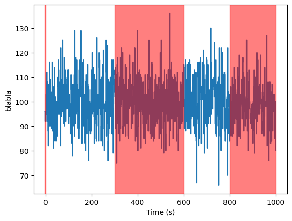
Plotting
A curve can be plotted with the plot method. Time intervals outside GTIs will be plotted as vertical red bands.
[51]:
ts.gti = np.asarray([[1, 300], [600, 800]])
ts.plot("blabla")
[51]:
<AxesSubplot: xlabel='Time (s)', ylabel='blabla'>
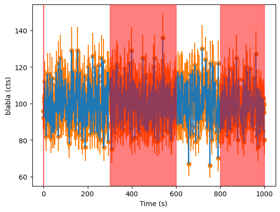
If a given array attr has an error bar (indicated by the attribute name + _err), one can specify witherrors=True to plot the attribute.
[52]:
ts.blabla_err = ts.blabla / 10.
ts.plot("blabla", labels=["Time (s)", "blabla (cts)"], witherrors=True)
[52]:
<AxesSubplot: xlabel='Time (s)', ylabel='blabla (cts)'>
A plot can also be customized using several keyword arguments.
[53]:
help(ts.plot)
Help on method plot in module stingray.base:

plot(attr, witherrors=False, labels=None, ax=None, title=None, marker='-', save=False, filename=None, plot_btis=True) method of stingray.base.StingrayTimeseries instance
    Plot the time series using ``matplotlib``.

    Plot the time series object on a graph ``self.time`` on x-axis and
    ``self.counts`` on y-axis with ``self.counts_err`` optionally
    as error bars.

    Parameters
    ----------
    attr: str
        Attribute to plot.

    Other parameters
    ----------------
    witherrors: boolean, default False
        Whether to plot the StingrayTimeseries with errorbars or not
    labels : iterable, default ``None``
        A list or tuple with ``xlabel`` and ``ylabel`` as strings. E.g.
        if the attribute is ``'counts'``, the list of labels
        could be ``['Time (s)', 'Counts (s^-1)']``
    ax : ``matplotlib.pyplot.axis`` object
        Axis to be used for plotting. Defaults to creating a new one.
    title : str, default ``None``
        The title of the plot.
    marker : str, default '-'
        Line style and color of the plot. Line styles and colors are
        combined in a single format string, as in ``'bo'`` for blue
        circles. See ``matplotlib.pyplot.plot`` for more options.
    save : boolean, optional, default ``False``
        If ``True``, save the figure with specified filename.
    filename : str
        File name of the image to save. Depends on the boolean ``save``.
    plot_btis : bool
        Plot the bad time intervals as red areas on the plot
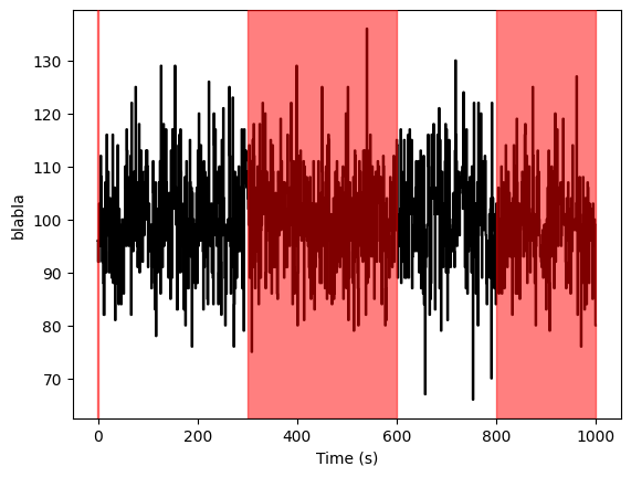
The figure drawn can also be saved in a file using keywords arguments in the plot method itself.
[54]:
ts.plot("blabla", marker = 'k', save=True, filename="lightcurve.png")
[54]:
<AxesSubplot: xlabel='Time (s)', ylabel='blabla'>
MJDREF and Shifting Times
The mjdref keyword argument defines a reference time in Modified Julian Date. Often, X-ray missions count their internal time in seconds from a given reference date and time (so that numbers don’t become arbitrarily large). The data is then in the format of Mission Elapsed Time (MET), or seconds since that reference time.
mjdref is generally passed into the Lightcurve object at instantiation, but it can be changed later:
[55]:
mjdref = 91254
time = np.arange(1000)
counts = np.random.poisson(100, size=len(time))

ts = StingrayTimeseries(time, array_attrs={"counts": counts}, dt=1, skip_checks=True, mjdref=mjdref)
print(ts.mjdref)
91254
[56]:
mjdref_new = mjdref - 20 / 86400  # Subtract 20 seconds from MJDREF
ts_new = ts.change_mjdref(mjdref_new)
print(ts_new.mjdref)
91253.99976851852
[57]:
ts_new.time
[57]:
array([  19.99999965,   20.99999965,   21.99999965,   22.99999965,
         23.99999965,   24.99999965,   25.99999965,   26.99999965,
         27.99999965,   28.99999965,   29.99999965,   30.99999965,
         31.99999965,   32.99999965,   33.99999965,   34.99999965,
         35.99999965,   36.99999965,   37.99999965,   38.99999965,
         39.99999965,   40.99999965,   41.99999965,   42.99999965,
         43.99999965,   44.99999965,   45.99999965,   46.99999965,
         47.99999965,   48.99999965,   49.99999965,   50.99999965,
         51.99999965,   52.99999965,   53.99999965,   54.99999965,
         55.99999965,   56.99999965,   57.99999965,   58.99999965,
         59.99999965,   60.99999965,   61.99999965,   62.99999965,
         63.99999965,   64.99999965,   65.99999965,   66.99999965,
         67.99999965,   68.99999965,   69.99999965,   70.99999965,
         71.99999965,   72.99999965,   73.99999965,   74.99999965,
         75.99999965,   76.99999965,   77.99999965,   78.99999965,
         79.99999965,   80.99999965,   81.99999965,   82.99999965,
         83.99999965,   84.99999965,   85.99999965,   86.99999965,
         87.99999965,   88.99999965,   89.99999965,   90.99999965,
         91.99999965,   92.99999965,   93.99999965,   94.99999965,
         95.99999965,   96.99999965,   97.99999965,   98.99999965,
         99.99999965,  100.99999965,  101.99999965,  102.99999965,
        103.99999965,  104.99999965,  105.99999965,  106.99999965,
        107.99999965,  108.99999965,  109.99999965,  110.99999965,
        111.99999965,  112.99999965,  113.99999965,  114.99999965,
        115.99999965,  116.99999965,  117.99999965,  118.99999965,
        119.99999965,  120.99999965,  121.99999965,  122.99999965,
        123.99999965,  124.99999965,  125.99999965,  126.99999965,
        127.99999965,  128.99999965,  129.99999965,  130.99999965,
        131.99999965,  132.99999965,  133.99999965,  134.99999965,
        135.99999965,  136.99999965,  137.99999965,  138.99999965,
        139.99999965,  140.99999965,  141.99999965,  142.99999965,
        143.99999965,  144.99999965,  145.99999965,  146.99999965,
        147.99999965,  148.99999965,  149.99999965,  150.99999965,
        151.99999965,  152.99999965,  153.99999965,  154.99999965,
        155.99999965,  156.99999965,  157.99999965,  158.99999965,
        159.99999965,  160.99999965,  161.99999965,  162.99999965,
        163.99999965,  164.99999965,  165.99999965,  166.99999965,
        167.99999965,  168.99999965,  169.99999965,  170.99999965,
        171.99999965,  172.99999965,  173.99999965,  174.99999965,
        175.99999965,  176.99999965,  177.99999965,  178.99999965,
        179.99999965,  180.99999965,  181.99999965,  182.99999965,
        183.99999965,  184.99999965,  185.99999965,  186.99999965,
        187.99999965,  188.99999965,  189.99999965,  190.99999965,
        191.99999965,  192.99999965,  193.99999965,  194.99999965,
        195.99999965,  196.99999965,  197.99999965,  198.99999965,
        199.99999965,  200.99999965,  201.99999965,  202.99999965,
        203.99999965,  204.99999965,  205.99999965,  206.99999965,
        207.99999965,  208.99999965,  209.99999965,  210.99999965,
        211.99999965,  212.99999965,  213.99999965,  214.99999965,
        215.99999965,  216.99999965,  217.99999965,  218.99999965,
        219.99999965,  220.99999965,  221.99999965,  222.99999965,
        223.99999965,  224.99999965,  225.99999965,  226.99999965,
        227.99999965,  228.99999965,  229.99999965,  230.99999965,
        231.99999965,  232.99999965,  233.99999965,  234.99999965,
        235.99999965,  236.99999965,  237.99999965,  238.99999965,
        239.99999965,  240.99999965,  241.99999965,  242.99999965,
        243.99999965,  244.99999965,  245.99999965,  246.99999965,
        247.99999965,  248.99999965,  249.99999965,  250.99999965,
        251.99999965,  252.99999965,  253.99999965,  254.99999965,
        255.99999965,  256.99999965,  257.99999965,  258.99999965,
        259.99999965,  260.99999965,  261.99999965,  262.99999965,
        263.99999965,  264.99999965,  265.99999965,  266.99999965,
        267.99999965,  268.99999965,  269.99999965,  270.99999965,
        271.99999965,  272.99999965,  273.99999965,  274.99999965,
        275.99999965,  276.99999965,  277.99999965,  278.99999965,
        279.99999965,  280.99999965,  281.99999965,  282.99999965,
        283.99999965,  284.99999965,  285.99999965,  286.99999965,
        287.99999965,  288.99999965,  289.99999965,  290.99999965,
        291.99999965,  292.99999965,  293.99999965,  294.99999965,
        295.99999965,  296.99999965,  297.99999965,  298.99999965,
        299.99999965,  300.99999965,  301.99999965,  302.99999965,
        303.99999965,  304.99999965,  305.99999965,  306.99999965,
        307.99999965,  308.99999965,  309.99999965,  310.99999965,
        311.99999965,  312.99999965,  313.99999965,  314.99999965,
        315.99999965,  316.99999965,  317.99999965,  318.99999965,
        319.99999965,  320.99999965,  321.99999965,  322.99999965,
        323.99999965,  324.99999965,  325.99999965,  326.99999965,
        327.99999965,  328.99999965,  329.99999965,  330.99999965,
        331.99999965,  332.99999965,  333.99999965,  334.99999965,
        335.99999965,  336.99999965,  337.99999965,  338.99999965,
        339.99999965,  340.99999965,  341.99999965,  342.99999965,
        343.99999965,  344.99999965,  345.99999965,  346.99999965,
        347.99999965,  348.99999965,  349.99999965,  350.99999965,
        351.99999965,  352.99999965,  353.99999965,  354.99999965,
        355.99999965,  356.99999965,  357.99999965,  358.99999965,
        359.99999965,  360.99999965,  361.99999965,  362.99999965,
        363.99999965,  364.99999965,  365.99999965,  366.99999965,
        367.99999965,  368.99999965,  369.99999965,  370.99999965,
        371.99999965,  372.99999965,  373.99999965,  374.99999965,
        375.99999965,  376.99999965,  377.99999965,  378.99999965,
        379.99999965,  380.99999965,  381.99999965,  382.99999965,
        383.99999965,  384.99999965,  385.99999965,  386.99999965,
        387.99999965,  388.99999965,  389.99999965,  390.99999965,
        391.99999965,  392.99999965,  393.99999965,  394.99999965,
        395.99999965,  396.99999965,  397.99999965,  398.99999965,
        399.99999965,  400.99999965,  401.99999965,  402.99999965,
        403.99999965,  404.99999965,  405.99999965,  406.99999965,
        407.99999965,  408.99999965,  409.99999965,  410.99999965,
        411.99999965,  412.99999965,  413.99999965,  414.99999965,
        415.99999965,  416.99999965,  417.99999965,  418.99999965,
        419.99999965,  420.99999965,  421.99999965,  422.99999965,
        423.99999965,  424.99999965,  425.99999965,  426.99999965,
        427.99999965,  428.99999965,  429.99999965,  430.99999965,
        431.99999965,  432.99999965,  433.99999965,  434.99999965,
        435.99999965,  436.99999965,  437.99999965,  438.99999965,
        439.99999965,  440.99999965,  441.99999965,  442.99999965,
        443.99999965,  444.99999965,  445.99999965,  446.99999965,
        447.99999965,  448.99999965,  449.99999965,  450.99999965,
        451.99999965,  452.99999965,  453.99999965,  454.99999965,
        455.99999965,  456.99999965,  457.99999965,  458.99999965,
        459.99999965,  460.99999965,  461.99999965,  462.99999965,
        463.99999965,  464.99999965,  465.99999965,  466.99999965,
        467.99999965,  468.99999965,  469.99999965,  470.99999965,
        471.99999965,  472.99999965,  473.99999965,  474.99999965,
        475.99999965,  476.99999965,  477.99999965,  478.99999965,
        479.99999965,  480.99999965,  481.99999965,  482.99999965,
        483.99999965,  484.99999965,  485.99999965,  486.99999965,
        487.99999965,  488.99999965,  489.99999965,  490.99999965,
        491.99999965,  492.99999965,  493.99999965,  494.99999965,
        495.99999965,  496.99999965,  497.99999965,  498.99999965,
        499.99999965,  500.99999965,  501.99999965,  502.99999965,
        503.99999965,  504.99999965,  505.99999965,  506.99999965,
        507.99999965,  508.99999965,  509.99999965,  510.99999965,
        511.99999965,  512.99999965,  513.99999965,  514.99999965,
        515.99999965,  516.99999965,  517.99999965,  518.99999965,
        519.99999965,  520.99999965,  521.99999965,  522.99999965,
        523.99999965,  524.99999965,  525.99999965,  526.99999965,
        527.99999965,  528.99999965,  529.99999965,  530.99999965,
        531.99999965,  532.99999965,  533.99999965,  534.99999965,
        535.99999965,  536.99999965,  537.99999965,  538.99999965,
        539.99999965,  540.99999965,  541.99999965,  542.99999965,
        543.99999965,  544.99999965,  545.99999965,  546.99999965,
        547.99999965,  548.99999965,  549.99999965,  550.99999965,
        551.99999965,  552.99999965,  553.99999965,  554.99999965,
        555.99999965,  556.99999965,  557.99999965,  558.99999965,
        559.99999965,  560.99999965,  561.99999965,  562.99999965,
        563.99999965,  564.99999965,  565.99999965,  566.99999965,
        567.99999965,  568.99999965,  569.99999965,  570.99999965,
        571.99999965,  572.99999965,  573.99999965,  574.99999965,
        575.99999965,  576.99999965,  577.99999965,  578.99999965,
        579.99999965,  580.99999965,  581.99999965,  582.99999965,
        583.99999965,  584.99999965,  585.99999965,  586.99999965,
        587.99999965,  588.99999965,  589.99999965,  590.99999965,
        591.99999965,  592.99999965,  593.99999965,  594.99999965,
        595.99999965,  596.99999965,  597.99999965,  598.99999965,
        599.99999965,  600.99999965,  601.99999965,  602.99999965,
        603.99999965,  604.99999965,  605.99999965,  606.99999965,
        607.99999965,  608.99999965,  609.99999965,  610.99999965,
        611.99999965,  612.99999965,  613.99999965,  614.99999965,
        615.99999965,  616.99999965,  617.99999965,  618.99999965,
        619.99999965,  620.99999965,  621.99999965,  622.99999965,
        623.99999965,  624.99999965,  625.99999965,  626.99999965,
        627.99999965,  628.99999965,  629.99999965,  630.99999965,
        631.99999965,  632.99999965,  633.99999965,  634.99999965,
        635.99999965,  636.99999965,  637.99999965,  638.99999965,
        639.99999965,  640.99999965,  641.99999965,  642.99999965,
        643.99999965,  644.99999965,  645.99999965,  646.99999965,
        647.99999965,  648.99999965,  649.99999965,  650.99999965,
        651.99999965,  652.99999965,  653.99999965,  654.99999965,
        655.99999965,  656.99999965,  657.99999965,  658.99999965,
        659.99999965,  660.99999965,  661.99999965,  662.99999965,
        663.99999965,  664.99999965,  665.99999965,  666.99999965,
        667.99999965,  668.99999965,  669.99999965,  670.99999965,
        671.99999965,  672.99999965,  673.99999965,  674.99999965,
        675.99999965,  676.99999965,  677.99999965,  678.99999965,
        679.99999965,  680.99999965,  681.99999965,  682.99999965,
        683.99999965,  684.99999965,  685.99999965,  686.99999965,
        687.99999965,  688.99999965,  689.99999965,  690.99999965,
        691.99999965,  692.99999965,  693.99999965,  694.99999965,
        695.99999965,  696.99999965,  697.99999965,  698.99999965,
        699.99999965,  700.99999965,  701.99999965,  702.99999965,
        703.99999965,  704.99999965,  705.99999965,  706.99999965,
        707.99999965,  708.99999965,  709.99999965,  710.99999965,
        711.99999965,  712.99999965,  713.99999965,  714.99999965,
        715.99999965,  716.99999965,  717.99999965,  718.99999965,
        719.99999965,  720.99999965,  721.99999965,  722.99999965,
        723.99999965,  724.99999965,  725.99999965,  726.99999965,
        727.99999965,  728.99999965,  729.99999965,  730.99999965,
        731.99999965,  732.99999965,  733.99999965,  734.99999965,
        735.99999965,  736.99999965,  737.99999965,  738.99999965,
        739.99999965,  740.99999965,  741.99999965,  742.99999965,
        743.99999965,  744.99999965,  745.99999965,  746.99999965,
        747.99999965,  748.99999965,  749.99999965,  750.99999965,
        751.99999965,  752.99999965,  753.99999965,  754.99999965,
        755.99999965,  756.99999965,  757.99999965,  758.99999965,
        759.99999965,  760.99999965,  761.99999965,  762.99999965,
        763.99999965,  764.99999965,  765.99999965,  766.99999965,
        767.99999965,  768.99999965,  769.99999965,  770.99999965,
        771.99999965,  772.99999965,  773.99999965,  774.99999965,
        775.99999965,  776.99999965,  777.99999965,  778.99999965,
        779.99999965,  780.99999965,  781.99999965,  782.99999965,
        783.99999965,  784.99999965,  785.99999965,  786.99999965,
        787.99999965,  788.99999965,  789.99999965,  790.99999965,
        791.99999965,  792.99999965,  793.99999965,  794.99999965,
        795.99999965,  796.99999965,  797.99999965,  798.99999965,
        799.99999965,  800.99999965,  801.99999965,  802.99999965,
        803.99999965,  804.99999965,  805.99999965,  806.99999965,
        807.99999965,  808.99999965,  809.99999965,  810.99999965,
        811.99999965,  812.99999965,  813.99999965,  814.99999965,
        815.99999965,  816.99999965,  817.99999965,  818.99999965,
        819.99999965,  820.99999965,  821.99999965,  822.99999965,
        823.99999965,  824.99999965,  825.99999965,  826.99999965,
        827.99999965,  828.99999965,  829.99999965,  830.99999965,
        831.99999965,  832.99999965,  833.99999965,  834.99999965,
        835.99999965,  836.99999965,  837.99999965,  838.99999965,
        839.99999965,  840.99999965,  841.99999965,  842.99999965,
        843.99999965,  844.99999965,  845.99999965,  846.99999965,
        847.99999965,  848.99999965,  849.99999965,  850.99999965,
        851.99999965,  852.99999965,  853.99999965,  854.99999965,
        855.99999965,  856.99999965,  857.99999965,  858.99999965,
        859.99999965,  860.99999965,  861.99999965,  862.99999965,
        863.99999965,  864.99999965,  865.99999965,  866.99999965,
        867.99999965,  868.99999965,  869.99999965,  870.99999965,
        871.99999965,  872.99999965,  873.99999965,  874.99999965,
        875.99999965,  876.99999965,  877.99999965,  878.99999965,
        879.99999965,  880.99999965,  881.99999965,  882.99999965,
        883.99999965,  884.99999965,  885.99999965,  886.99999965,
        887.99999965,  888.99999965,  889.99999965,  890.99999965,
        891.99999965,  892.99999965,  893.99999965,  894.99999965,
        895.99999965,  896.99999965,  897.99999965,  898.99999965,
        899.99999965,  900.99999965,  901.99999965,  902.99999965,
        903.99999965,  904.99999965,  905.99999965,  906.99999965,
        907.99999965,  908.99999965,  909.99999965,  910.99999965,
        911.99999965,  912.99999965,  913.99999965,  914.99999965,
        915.99999965,  916.99999965,  917.99999965,  918.99999965,
        919.99999965,  920.99999965,  921.99999965,  922.99999965,
        923.99999965,  924.99999965,  925.99999965,  926.99999965,
        927.99999965,  928.99999965,  929.99999965,  930.99999965,
        931.99999965,  932.99999965,  933.99999965,  934.99999965,
        935.99999965,  936.99999965,  937.99999965,  938.99999965,
        939.99999965,  940.99999965,  941.99999965,  942.99999965,
        943.99999965,  944.99999965,  945.99999965,  946.99999965,
        947.99999965,  948.99999965,  949.99999965,  950.99999965,
        951.99999965,  952.99999965,  953.99999965,  954.99999965,
        955.99999965,  956.99999965,  957.99999965,  958.99999965,
        959.99999965,  960.99999965,  961.99999965,  962.99999965,
        963.99999965,  964.99999965,  965.99999965,  966.99999965,
        967.99999965,  968.99999965,  969.99999965,  970.99999965,
        971.99999965,  972.99999965,  973.99999965,  974.99999965,
        975.99999965,  976.99999965,  977.99999965,  978.99999965,
        979.99999965,  980.99999965,  981.99999965,  982.99999965,
        983.99999965,  984.99999965,  985.99999965,  986.99999965,
        987.99999965,  988.99999965,  989.99999965,  990.99999965,
        991.99999965,  992.99999965,  993.99999965,  994.99999965,
        995.99999965,  996.99999965,  997.99999965,  998.99999965,
        999.99999965, 1000.99999965, 1001.99999965, 1002.99999965,
       1003.99999965, 1004.99999965, 1005.99999965, 1006.99999965,
       1007.99999965, 1008.99999965, 1009.99999965, 1010.99999965,
       1011.99999965, 1012.99999965, 1013.99999965, 1014.99999965,
       1015.99999965, 1016.99999965, 1017.99999965, 1018.99999965])
[58]:
ts_new.gti
[58]:
array([[ 19.49999965, 1019.49999965]])
This changes the reference time and all the times referred to it. It’s very useful when manipulating time series from different missions. Alternatively, one can shift the times (by a value in seconds) without modifying the MJDREF
[59]:
gti = [(0,500), (600, 1000)]
ts.gti = gti
[60]:
print("first three time bins: " + str(ts.time[:3]))
print("GTIs: " + str(ts.gti))
first three time bins: [0 1 2]
GTIs: [[   0  500]
 [ 600 1000]]
[61]:
time_shift = 10.0
ts_shifted = ts.shift(time_shift)
[62]:
print("Shifted first three time bins: " + str(ts_shifted.time[:3]))
print("Shifted GTIs: " + str(ts_shifted.gti))
Shifted first three time bins: [10. 11. 12.]
Shifted GTIs: [[  10.  510.]
 [ 610. 1010.]]
Splitting by GTI
A special case of splitting your light curve object is to split by GTIs. This can be helpful if you want to look at individual contiguous segments separately:
[63]:
# make a time array with a big gap and a small gap
time = np.arange(20)
counts = np.random.poisson(100, size=len(time))
gti = [(0,8), (12,20)]


ts = StingrayTimeseries(time, array_attrs={"blabla": counts}, dt=1, gti=gti)
[64]:
ts_split = ts.split_by_gti()
[65]:
print(ts.time, ts.blabla)
for ts_tmp in ts_split:
    print(ts_tmp.time, ts_tmp.blabla)
[ 0  1  2  3  4  5  6  7  8  9 10 11 12 13 14 15 16 17 18 19] [102  97  95 105 100  96 107 119  94 119 101  91 104  89 119 106 111  89
 100 110]
[1 2 3 4 5 6 7] [ 97  95 105 100  96 107 119]
[13 14 15 16 17 18 19] [ 89 119 106 111  89 100 110]
Because I’d passed in GTIs that define the range from 0-8 and from 12-20 as good time intervals, the light curve will be split into two individual ones containing all data points falling within these ranges.
You can also apply the GTIs directly to the original light curve, which will filter time, counts, countrate, counts_err and countrate_err to only fall within the bounds of the GTIs:
[66]:
# make a time array with a big gap and a small gap
time = np.arange(20)
counts = np.random.poisson(100, size=len(time))
gti = [(0,8), (12,20)]


ts = StingrayTimeseries(time, array_attrs={"blabla": counts}, dt=1, gti=gti)
Caution: This is one of the few methods that change the original state of the object, rather than returning a new copy of it with the changes applied! So any events falling outside of the range of the GTIs will be lost:
[67]:
# time array before applying GTIs:
ts.time
[67]:
array([ 0,  1,  2,  3,  4,  5,  6,  7,  8,  9, 10, 11, 12, 13, 14, 15, 16,
       17, 18, 19])
[68]:
ts.apply_gtis()
[68]:
<stingray.base.StingrayTimeseries at 0x13bb33c70>
[69]:
# time array after applying GTIs
ts.time
[69]:
array([ 1, 2, 3, 4, 5, 6, 7, 13, 14, 15, 16, 17, 18, 19])
As you can see, the time bins 8-12 have been dropped, since they fall outside of the GTIs.
Reading/Writing Stingray Timeseries to/from files
The StingrayTimeseries class has roundtrip reading/writing capabilities via the read and write methods. Most of the I/O is managed by the astropy.io infrastructure. We regularly test the roundtrip to Enhanced CSV (.ecsv) and Hierarchical Data Format v.5 (.hdf5) formats.
Converting StingrayTimeseries to pandas, xarray and Astropy Table/Timeseries
StingrayTimeseries can be converted back and forth to xarray, pandas, astropy.table.Table and astropy.timeseries.TimeSeries objects through the relevant to_FORMAT and from_FORMAT, e.g. Refer to the methods’ documentation for more information on how data are stored in each case.
[70]:
type(ts.to_pandas())
[70]:
pandas.core.frame.DataFrame
[71]:
type(ts.to_xarray())
[71]:
xarray.core.dataset.Dataset
[72]:
type(ts.to_astropy_table())
[72]:
astropy.table.table.Table
[73]:
type(ts.to_astropy_timeseries())
[73]:
astropy.timeseries.sampled.TimeSeries
[ ]: