Fourier Amplitude Difference correction in Stingray

%load_ext autoreload
%autoreload 2
import numpy as np
import matplotlib.pyplot as plt
from stingray import EventList, AveragedCrossspectrum, AveragedPowerspectrum
from stingray.deadtime.fad import calculate_FAD_correction, FAD
from stingray.filters import filter_for_deadtime

import matplotlib.pyplot as plt

Dead time affects most counting experiments. While the instrument is busy processing one event, it is “dead” to other photons/particles hitting the detector. This is usually not an issue if the count rate is low enough, or the processing time (dead time) is small enough. However, at high count rate dead time affects greatly the statistical properties of the data, to a point where a standard periodicity search based on the periodogram/power density spectrum (PDS) cannot be carried out.

The Fourier Amplitude Difference (FAD) correction is described in Bachetti & Huppenkothen, 2018, ApJ, 853L, 21, and is able to correct precisely deadtime affected PDSs if we have at least two identical and independent detectors. This is common in new generation X-ray timing instruments, often based on multiple-detector configurations (e.g. NuSTAR, NICER, AstroSAT, etc.).

In the code below, we calculate the PDS of light curves without dead time, after applying a dead time filter, and after applying the FAD to the dead-time affected dataset.

def generate_events(length, ncounts):
    ev = np.random.uniform(0, length, ncounts)
    ev.sort()
    return ev

ctrate = 500
dt = 0.001
deadtime = 2.5e-3
tstart = 0
length = 25600
segment_size = 256.
ncounts = int(ctrate * length)
ev1 = EventList(generate_events(length, ncounts), mjdref=58000, gti=[[tstart, length]])
ev2 = EventList(generate_events(length, ncounts), mjdref=58000, gti=[[tstart, length]])

pds1 = AveragedPowerspectrum.from_events(ev1, dt=dt, segment_size=segment_size, norm='leahy')
pds2 = AveragedPowerspectrum.from_events(ev2, dt=dt, segment_size=segment_size, norm='leahy')
ptot = AveragedPowerspectrum.from_events(ev1.join(ev2), dt=dt, segment_size=segment_size, norm='leahy')
cs = AveragedCrossspectrum.from_events(ev1, ev2, dt=dt, segment_size=segment_size, norm='leahy')

100it [00:01, 98.20it/s]
100it [00:00, 134.62it/s]
100it [00:01, 80.61it/s]
100it [00:01, 52.97it/s]

Now let us apply a deadtime filter to the events generated above, and calculate the corresponding periodograms

ev1_dt = ev1.apply_deadtime(deadtime)
ev2_dt = ev2.apply_deadtime(deadtime)

pds1_dt = AveragedPowerspectrum.from_events(ev1_dt, dt=dt, segment_size=segment_size, norm='leahy')
pds2_dt = AveragedPowerspectrum.from_events(ev2_dt, dt=dt, segment_size=segment_size, norm='leahy')
ptot_dt = AveragedPowerspectrum.from_events(ev1_dt.join(ev2_dt), dt=dt, segment_size=segment_size, norm='leahy')
cs_dt = AveragedCrossspectrum.from_events(ev1_dt, ev2_dt, dt=dt, segment_size=segment_size, norm='leahy')

100it [00:00, 154.30it/s]
100it [00:00, 167.20it/s]
100it [00:00, 133.60it/s]
100it [00:01, 67.74it/s]

The FAD method relies on averaging out many values of the difference between the Fourier transforms in the two channels in contiguous frequencies, and it works best when the frequency resolution is very high compared with the distortion of the power spectrum due to deadtime.

For example, in NuSTAR the effect of deadtime appears above \(\sim10\) Hz. We want to calculate the correction on a Hz-by-Hz basis, so that the correction is adequate. The frequency resolution from the FFT is 1/segment_size.

Therefore, the ``segment_size`` should ideally be some hundred seconds to have some hundred bins in a Hz. The smoothing length should be of the order of the number of bins in \(\sim1\) Hz (in this example 2Hz).

results = \
    FAD(ev1_dt, ev2_dt, segment_size, dt, norm="leahy", plot=False,
                      smoothing_alg='gauss',
                      smoothing_length=segment_size*2,
                      strict=True, verbose=False,
                      tolerance=0.05)

freq_f = results['freq']
pds1_f = results['pds1']
pds2_f = results['pds2']
cs_f = results['cs']
ptot_f = results['ptot']

100it [00:33,  2.99it/s]

M: 100

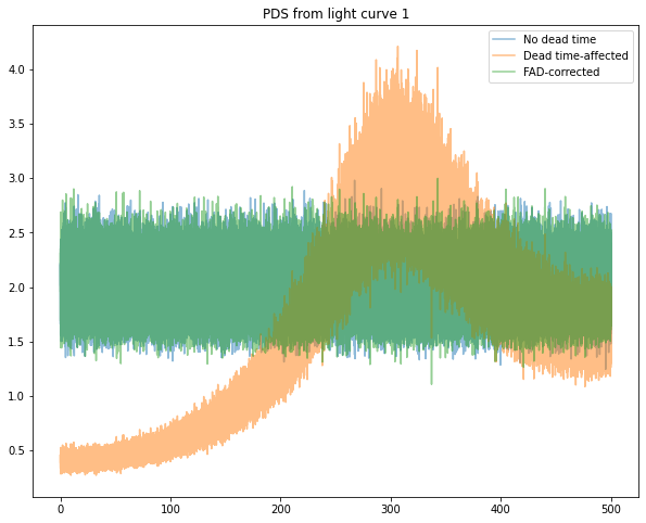
for spec, spec_dt, spec_f, label in zip(
        [pds1, pds1, ptot, cs],
        [pds1_dt, pds2_dt, ptot_dt, cs_dt],
        [pds1_f, pds2_f, ptot_f, cs_f],
        ['PDS from light curve 1', 'PDS from light curve 2', 'PDS from lcs 1+2', 'cospectrum']
        ):
    plt.figure(figsize=(10, 8))
    plt.title(label)
    plt.plot(spec.freq, spec.power, label='No dead time', alpha=0.5)
    plt.plot(spec_dt.freq, spec_dt.power, label='Dead time-affected', alpha=0.5)
    plt.plot(freq_f, spec_f, label='FAD-corrected', alpha=0.5)
    plt.legend()

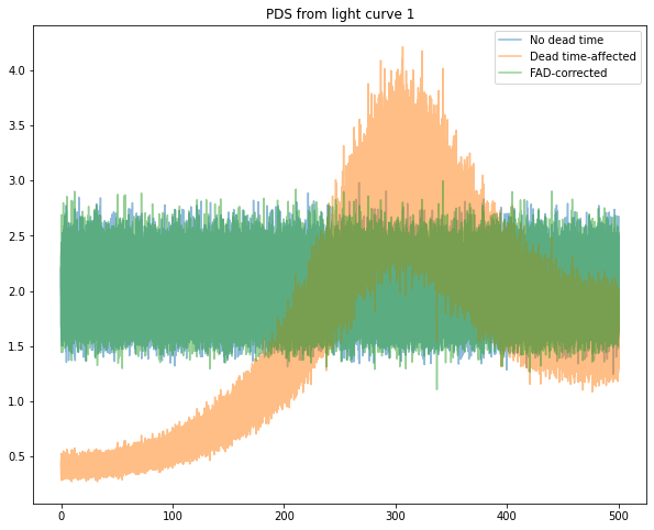
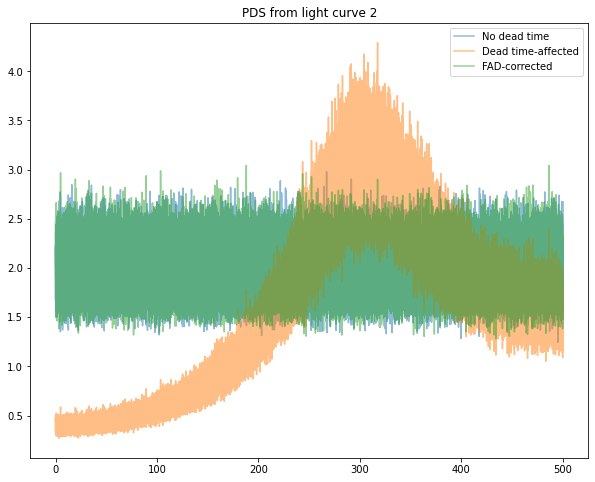
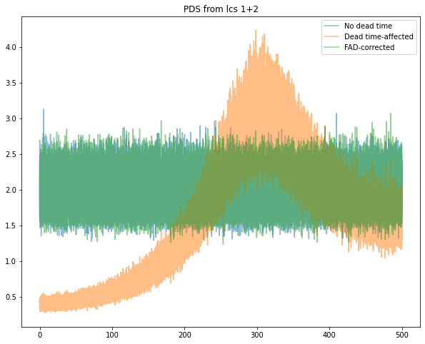
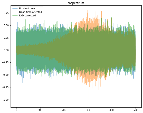
As can be seen above, all power density and co- spectra have been corrected accurately in their basic property (the white noise level). See Bachetti & Huppenkothen 2019 for more information.

Note that this can also be done starting from light curves:

# Calculate light curves
lc1_dt = ev1_dt.to_lc(dt=dt)
lc2_dt = ev2_dt.to_lc(dt=dt)

results = \
    FAD(lc1_dt, lc2_dt, segment_size, dt, norm="leahy", plot=False,
                      smoothing_alg='gauss',
                      smoothing_length=segment_size*2,
                      strict=True, verbose=False,
                      tolerance=0.05)

freq_f = results['freq']
pds1_f = results['pds1']
pds2_f = results['pds2']
cs_f = results['cs']
ptot_f = results['ptot']

for spec, spec_dt, spec_f, label in zip(
        [pds1, pds1, ptot, cs],
        [pds1_dt, pds2_dt, ptot_dt, cs_dt],
        [pds1_f, pds2_f, ptot_f, cs_f],
        ['PDS from light curve 1', 'PDS from light curve 2', 'PDS from lcs 1+2', 'cospectrum']
        ):
    plt.figure(figsize=(10, 8))
    plt.title(label)
    plt.plot(spec.freq, spec.power, label='No dead time', alpha=0.5)
    plt.plot(spec_dt.freq, spec_dt.power, label='Dead time-affected', alpha=0.5)
    plt.plot(freq_f, spec_f, label='FAD-corrected', alpha=0.5)
    plt.legend()

100it [00:34,  2.93it/s]

M: 100